Can you train a text-to-image model without any text?
Despite Betteridge’s law, I contend the answer is “probably”. I’d prefer to be writing a post without a question mark at the end of the title, but I haven’t actually gotten it to work yet. This post is something of a research log documenting my efforts, though written ex post. This code for the models and data processing is here.
Why should it be possible?
A text-to-image model is one which, well, takes in text and outputs images. DALL-E and Midjourney are the most famous examples, but there are tons. The user types in a prompt (“Central Park during the freak snowstorm of 2024, shot on Hasselblad medium format”) and the model generates an image that resembles the prompt. They’re trained on pairs of captions and images, so the objective is more like an image that would have that caption. The modern wave was kicked off by DALL-E and to a greater extent CLIP. Most of the open source models I’ve seen exploit CLIP in some way, and the proprietary ones probably do too. It should, in my opinion, be possible to use CLIP and an unlabeled set of images to make a text-to-image model.
CLIP was released back in January 2021. It’s a model that associates images and captions. Both images and captions are projected into a shared vector space and the training objective is to maximize the cosine similarity between images and their captions1. This training objective, plus lots of data and compute, results in a model that knows a ton about images. It can identify locations, famous people, objects, animals, and do them in combination. This web app lets you search the LAION-5B dataset using CLIP. It’s unfortunately down right now, but maybe you’ll be lucky and it’ll be up when you read this. As an illustration of the power of CLIP, the results will dramatically change if you tack “shot with Sony a7R” (or some other camera) onto the end of a query that returns photos. People who label their photos with what type of camera they used take different types of photos from people who don’t, and people who use different cameras take different types of photos from each other. CLIP knows this. And it works for image to image comparisons as well - a picture of the Golden Gate Bridge’s embedding will have high cosine similarity to other pictures of the Golden Gate, regardless of angle, weather, time of day, etc. Even paintings and drawings will match.
So, since CLIP knows what labels go with which images, you shouldn’t need labels of your own to train a text-to-image model. You should be able to entirely rely on CLIP for the supervision. That’s the goal.
A baseline
My first attempt simply conditioned image generation on the CLIP embeddings of the images. This works, you can input an image(’s embedding) and get a similar image out. The model learns the inverse of CLIP’s image projection function. But if you input a text embedding instead, things are not so rosy.
Here’s 100 samples from the baseline model conditioned on a photo of a friend of mine. In the photo she has a sideshave, with the hair on her left side shaved and the hair on her right long. I think that’s why so many of the samples have the head tilted to the model’s right. She’s also wearing glasses in the prompt image, which is why so many of the samples have glasses.

That’s the level of image quality you get from 25M images and 8 4090s for 82 hours2. Good enough for proof of concept, but not more. The two things my models are best at are faces and screenshots of GTA. Here are 100 samples conditioned on a GTA screenshot from the dataset.

So, at least on image prompts, this baseline model works. Let’s try a couple matched text prompts. Here’s “A woman’s face”:

And here’s “A screenshot of Grand Theft Auto”:

It generates faces, but they’re distorted, expressionless, posed weirdly, and sometimes off color. As for the GTA screenshot prompt, none of them look like GTA screenshots. They look like photos taken outdoors, and if we squint a bit we can see a lot of what might be cars. It’s much better at image prompts than it is at text prompts. Here’s the theory of why this should be the case:
The CLIP embeddings of images and captions are drawn from different distributions. CLIP’s objective puts images and reasonable captions for them close together, but that doesn’t mean they need to be on top of each other. An image’s embedding needs to be close to many possible captions’ embeddings simultaneously, and those caption embeddings need to be different so that they can be closer or further from different images. E.g. the photo of my friend’s embedding should be close to “a woman’s face”, “new haircut”, “day 2 at Burning Man”, etc. And since those emphasize different aspects of the photo, they should be separated. “A woman’s face” shouldn’t be closer to sideshaves than anything else, “day 2 at Burning Man” doesn’t necessarily need to be closer to images of people than images of sculptures, but does need to be near images that are in a dusty grey-orange place and far from forests or offices.
Furthermore, a model that learns to invert CLIP’s image projection function perfectly would generate images that had exactly the input CLIP embedding, which isn’t what you want. Instead you want images that are reasonably close to the input, for some definition of “reasonably close”.
Conditioning on a range
I went through several variations trying to get this to work. The first set worked at training time. The training code would choose either a range of distances or a concrete distance (depending on which version of the code we’re talking about), then sample a point with a cosine distance to the actual embedding within that range or with that distance from the real image embedding, and use that as conditioning data. This approach makes text embeddings in-distribution (provided the distances we choose cover the distance away captions tend to be), and the model should learn to generate ranges, but the distribution of images conditional on the range or distance is not what you want. Ideally the conditional distribution would be uniform over the possible images that have embeddings contained within the range, but a scheme that generates conditioning data based on the embeddings implicitly creates a distribution over the embeddings and not over the images. To make the distributions shaped like you want, you have to generate the conditioning data ahead of time and sample training images uniformly from the set that are inside the range.
Spherical caps in CLIP space
If we rephrase the “range” as a spherical cap, we can use the mathematical language that already exists to talk about them. (And talk to ChatGPT about them.) A spherical cap is a region of an (n-dimensional) sphere that is within some maximum angular distance from a vector. Since CLIP embeddings are unit vectors in 768-d space, we can define segments of CLIP space as caps. We have a central point in CLIP space and a maximum cosine distance, (defining the cap in terms of maximum angle or minimum cosine similarity is equivalent). Prompting the model with a cap centered on some point should generate images that are a maximum “semantic” distance from that point. So e.g. if you prompt the model with a cap centered on the embedding of the face above, a small maximum cosine distance should get you very similar images, and a larger maximum cosine distance should get you images that are still photos of faces, but not necessarily a similar looking person, a similar angle, light, etc. And a maximum cosine distance of 2 (covering the whole sphere) should be equivalent to unconditional sampling of the full distribution. A similar cap centered on the embedding of “The Golden Gate Bridge at sunset” should get you images that are pictures of the Golden Gate, but depending on the size of the cap, they might not be at sunset, or they might not be of that specific bridge. In addition, it’s important to note that the cosine distances between image embeddings and text embeddings don’t go below like 0.55. Even a very aligned image and caption are pretty far apart in CLIP space.
Sampling from the subset of a discrete set of unit vectors contained within a spherical cap
Since I’d decided I needed to generate caps and sample images from the training set that have embeddings within them, I needed to write software to do this. It was exceedingly difficult to do this efficiently. My run generating 25M cap-image pairs took around 4 days. And that’s after a lot of optimization effort. It runs at like 20-25% GPU utilization. So there’s a lot of room for improvement (I sure as hell hope so anyway). One should not write high performance code that needs to do a lot of work on the CPU as well as the GPU in Python. Or using JAX, probably. If I ever get around to doing a rewrite it’ll be in Rust and deal with the GPU at a lower level. Anyway, notes on what I did do:
A space partitioning data structure for unit vectors
I organize the vectors into a tree of spherical caps. Each tree contains a set of vectors, a central vector, and a maximum cosine distance. Every vector has a cosine distance to the central vector less than or equal to the maximum cosine distance. Leaves directly contain vectors, and nodes contain a set of k children, where k is a configurable integer constant >= 2 (in practice 64 or 128). Initially, the tree consists of a single leaf which has an arbitrary center and a maximum cosine distance of 2 (the opposite side of the sphere). Then, leaves are split recursively until all leaves are smaller than some configurable maximum number of vectors.
To split a leaf into a node and a set of children, I do k-means on the vectors in the leaf. The centroids become the children’s central vectors, and the maximum cosine distances are computed by iterating over the vectors in the children. Leaves are split until they contain less than some configurable maximum number of vectors.
I call this structure a captree. This structure has two important properties for sampling. First, you can test whether two caps intersect, and whether one contains the other, based only on the cap geometry. When sampling vectors in a captree that are contained within a query cap, you can eliminate any subtrees from consideration whose caps don’t intersect the query cap; if the query cap contains the entire cap of a subtree, then you can skip looking inside that subtree. Second, clustering the vectors at the top level means matching vectors are more likely in some subtrees than others, which makes approximate sampling work better.
Aside: Infinidata
The CLIP embeddings of my 25M image dataset are ~72GiB. That doesn’t fit in RAM on my home machine, though it does fit on bigger servers. I wrote a library for manipulating big datasets that don’t fit in RAM called Infinidata. Initially, I tried to use Huggingface’s Datasets library, but it was way too slow and ate tons of RAM and disk space. In general, Datasets is fine if you’re just downloading stuff, shuffling stuff, loading stuff or iterating over it in batches, but there’s all this other functionality and I get the vibe that nobody seriously uses it. Infinidata allows me to do the leaf splitting operation without copying while keeping the vectors out of RAM.
Two stage sampling
Sampling proceeds in two phases, an approximate algorithm that works on ~80% of queries and an exact algorithm that works on the remainder, is much slower, and takes the majority of the overall runtime.
The approximate sampling algorithm operates non-recursively at the top node and proceeds by estimating the number of vectors in each immediate child subtree that are contained within the query cap. First it computes the intersection status of each child’s cap with the query cap. Children that are fully contained by the query naturally have all of their vectors match, and children that don’t intersect have zero matches. For children that intersect the query cap but are not contained by it, we estimate the number of matching vectors by sampling uniformly inside that child. Our estimate is the fraction of samples that match times the number of vectors in the child. Once estimates have been computed for all children, we sample from the children in proportion to their estimates. For the fully contained children we sample from all their vectors, and for the intersecting children we sample from the matching vectors that we sampled from to estimate the number of matches. The number of samples used for density estimation is a tradeoff between sampling time, bias, and, when doing batched sampling, duplicate rate.
If the approximate sampling algorithm finds zero matches, sampling falls back to an exact algorithm. If we were willing to accept false negatives we could skip it, but it’s important in this application for the training examples to include small caps that contain few or one vectors. Exact sampling works by enumerating the matches in every subtree and sampling from them. This is conceptually straightforward. A lot of engineering effort went into making the vector checks asynchronous, batching, and various microoptimzations. Python is not a fast language, and dumb stuff like accessing a foo.length property directly instead of calling len(foo) can make a big difference.
Batched sampling
A lot of the costs of sampling can be amortized across multiple queries. In approximate sampling you can share the density estimation samples across queries, and in exact sampling the work of loading the vectors in leaves and shipping them to the GPU can be shared. This stuff makes a huge difference and is necessary to make sampling performance at all tolerable.
Generating the caps to sample from
CLIP space is large and high dimensional, and we want some of our caps to be very small. This means that generating caps with uniformly distributed centers is untenable - the vast majority of the small caps will be empty, meaning the generated training examples would disproportionately have large sizes. My approach is this is simple: to generate a cap I sample two vectors from the set of embeddings we’re generating from, generate a value in U[0, 1], and do spherical linear interpolation between the two vectors, using the value as the interpolation parameter. To get more useful conditioning data, I draw the maximum cosine distances non-uniformly. 95% of the time they’re drawn from U[0, 1], the remaining 5% of the time they’re drawn from U[1, 2]. Since users are mostly going to use the model with distances below 1, and since smaller caps provide more information at training time, this seems like a good idea. Given the results discussed below it’s hard to tell whether this achieves the goals, but it’s simple and seems logically sound.
Cap conditioned results
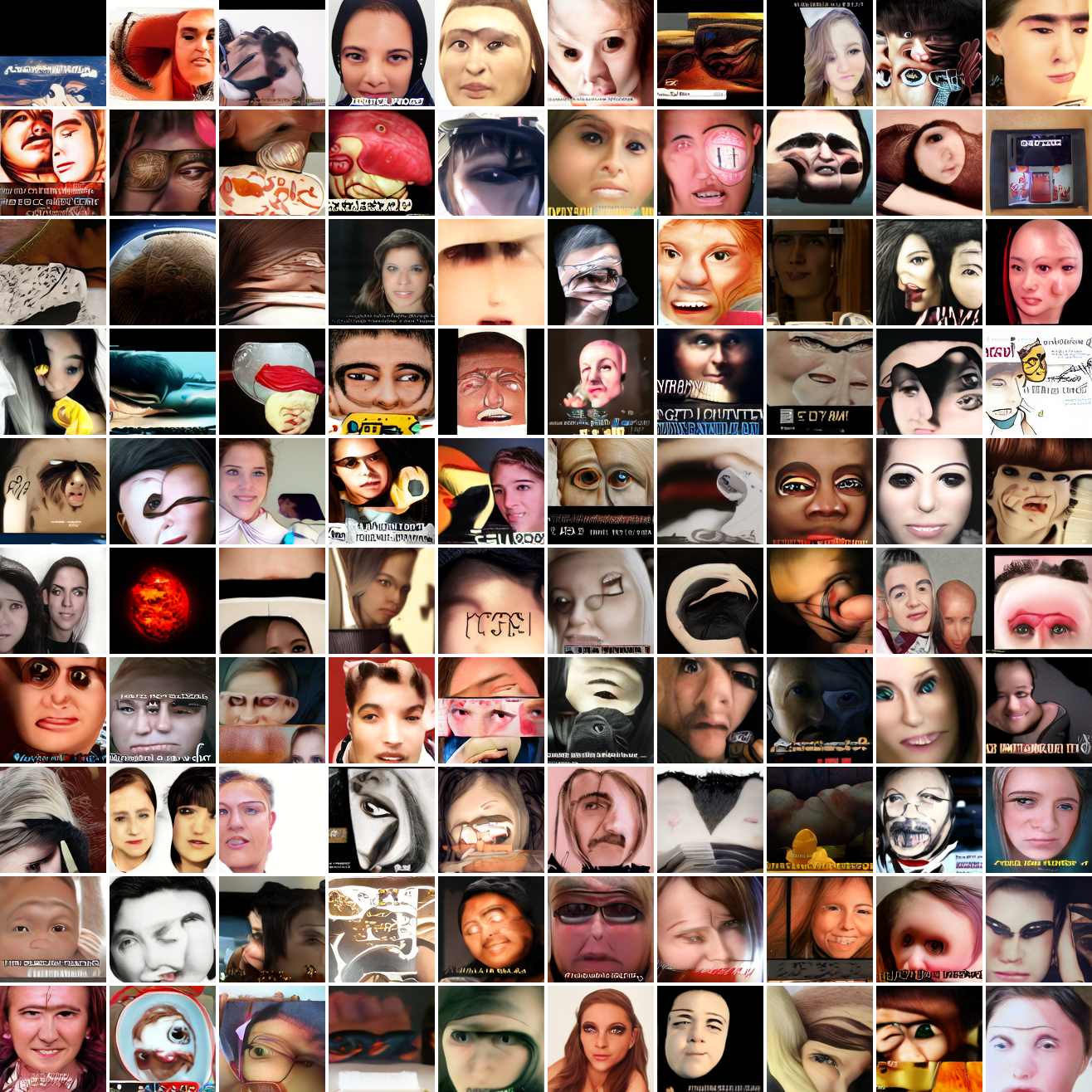
My cap conditioned model achieves losses very close to the baseline model, but the samples are not as good as one would hope. Here’s a series of images conditioned on the embedding of the same photo of my friend, with max cosine distances from 2.0 (the entirety of CLIP space) to 0.0 (a point). Note that the surface areas of these caps is nonlineary related to the max cosine distance. The surface area is heavily concentrated near the middle when working in high dimensions - while the cap with max distance 2.0 covers the entire sphere and the cap with max distance 1.0 covers half the sphere, the cap with max distance 0.5 covers way less than a quarter of the sphere.
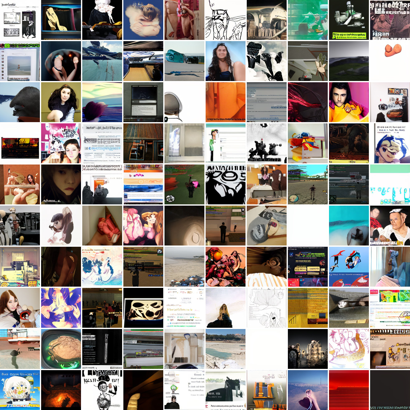
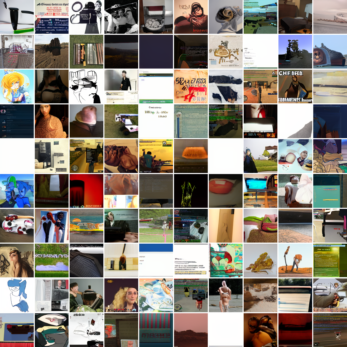
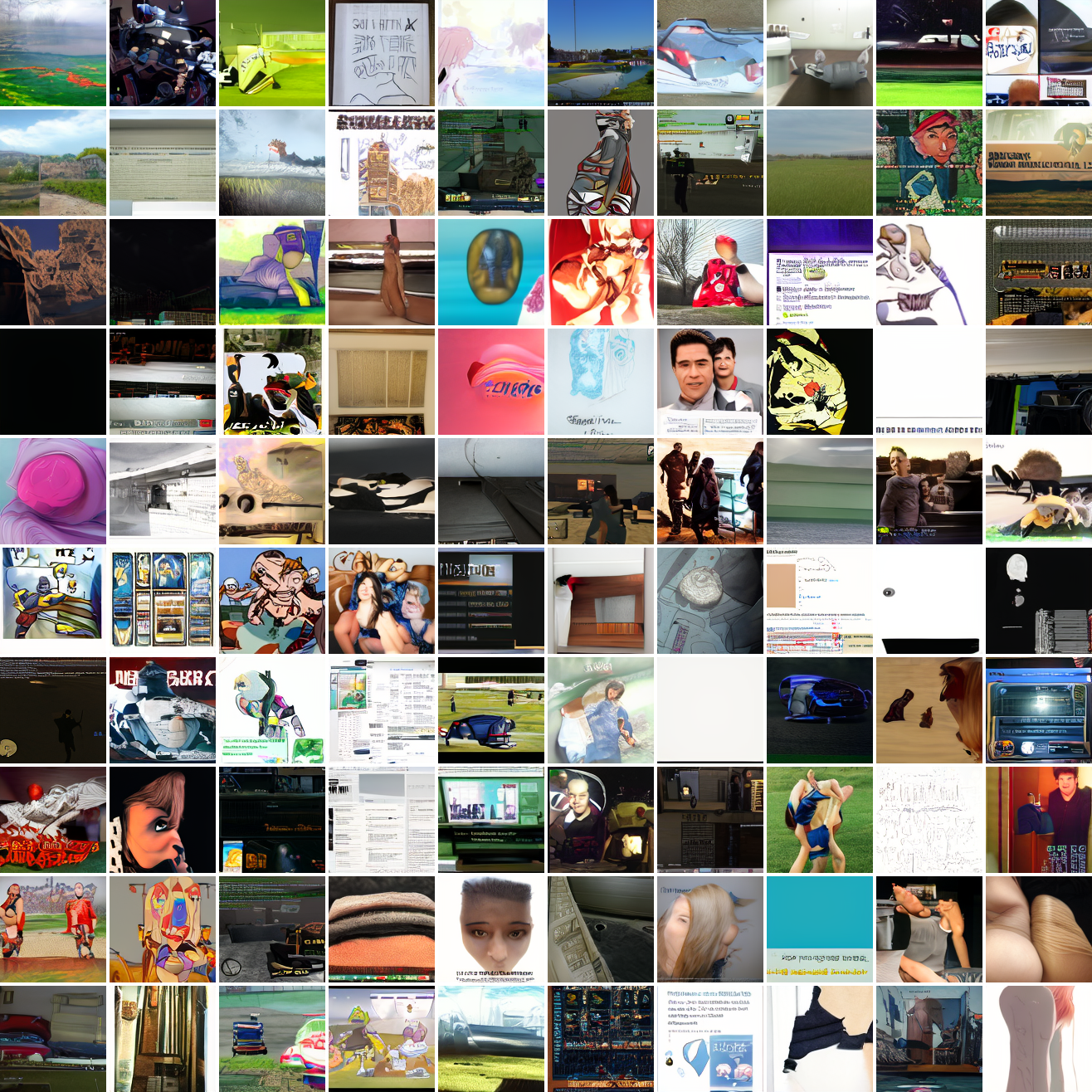
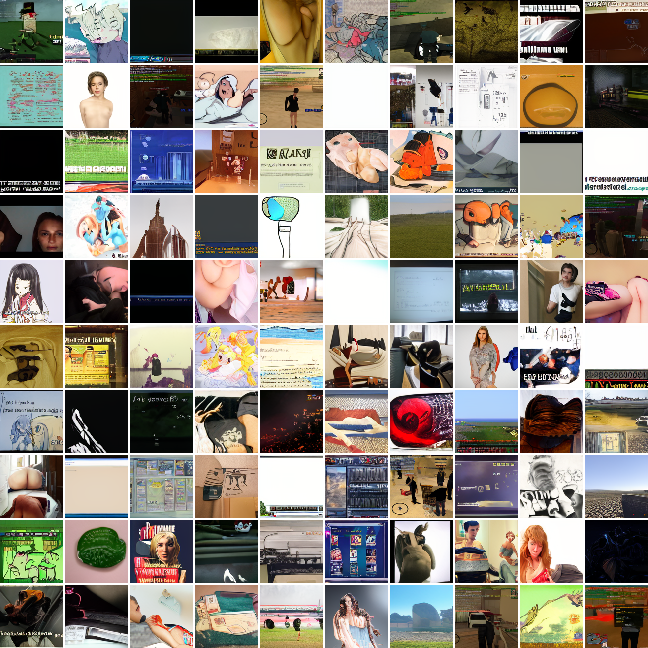
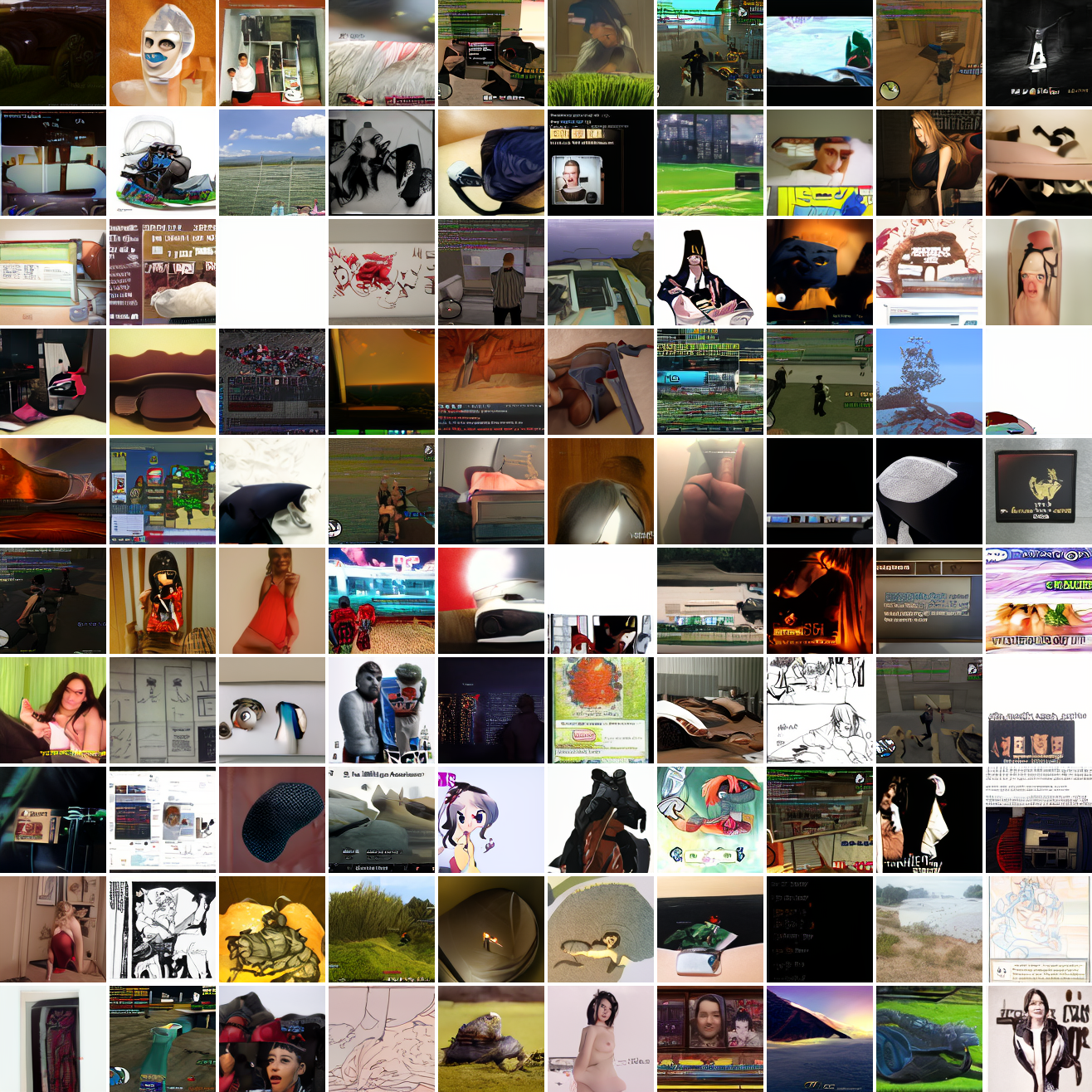
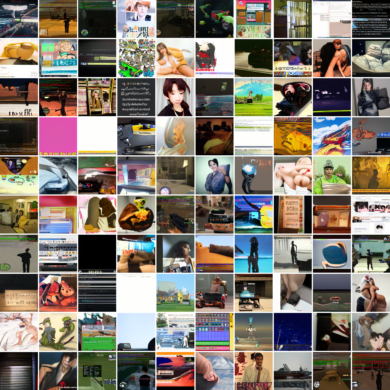
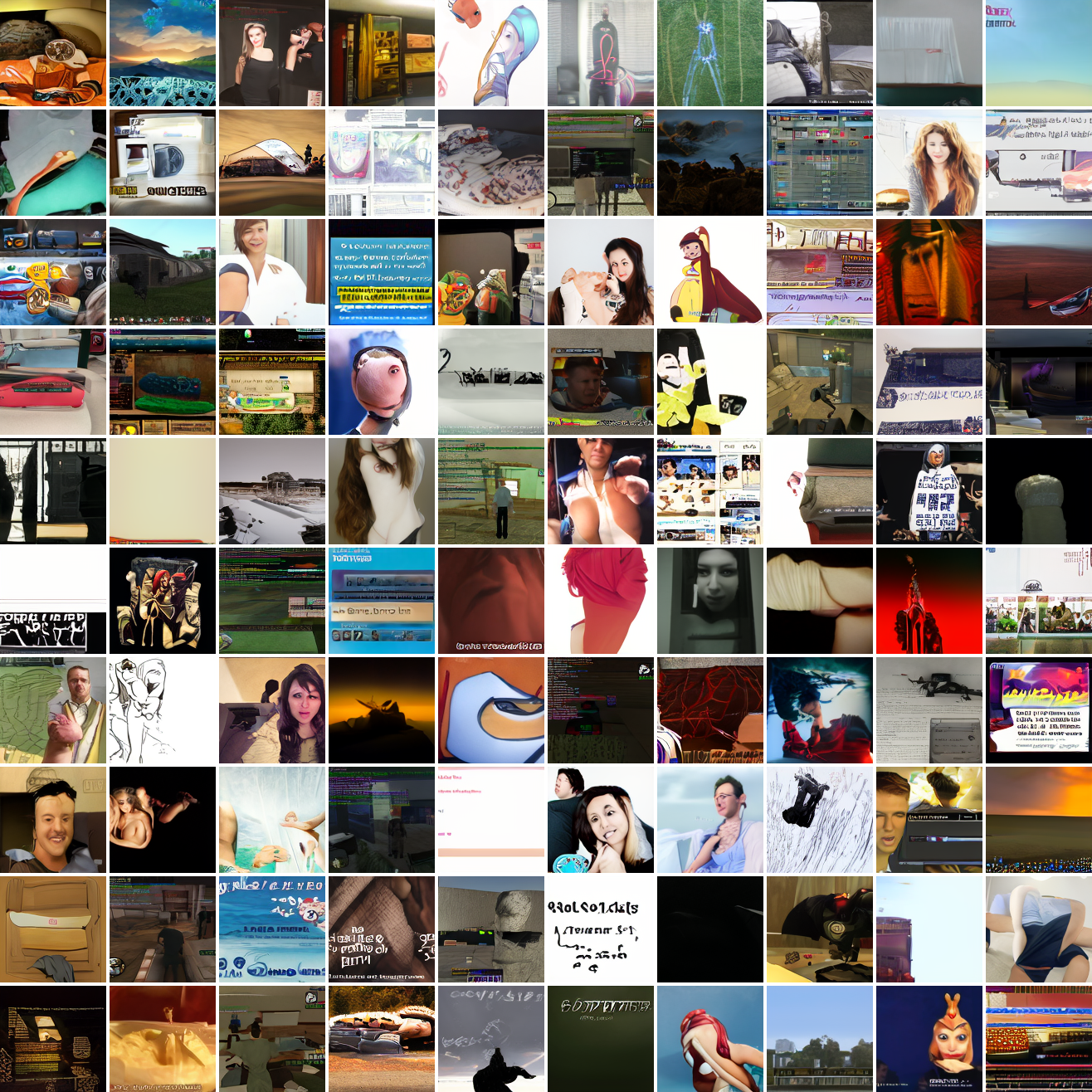
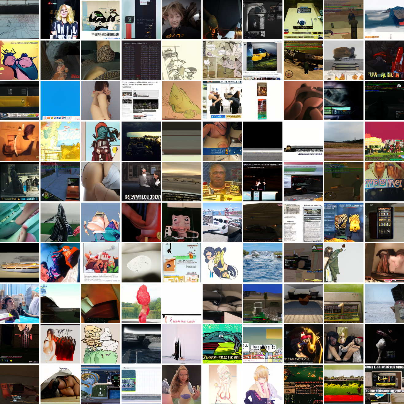
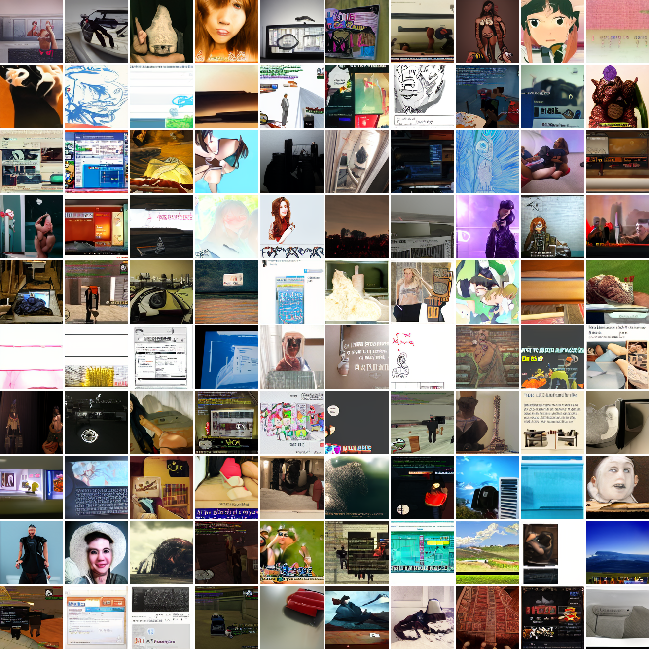
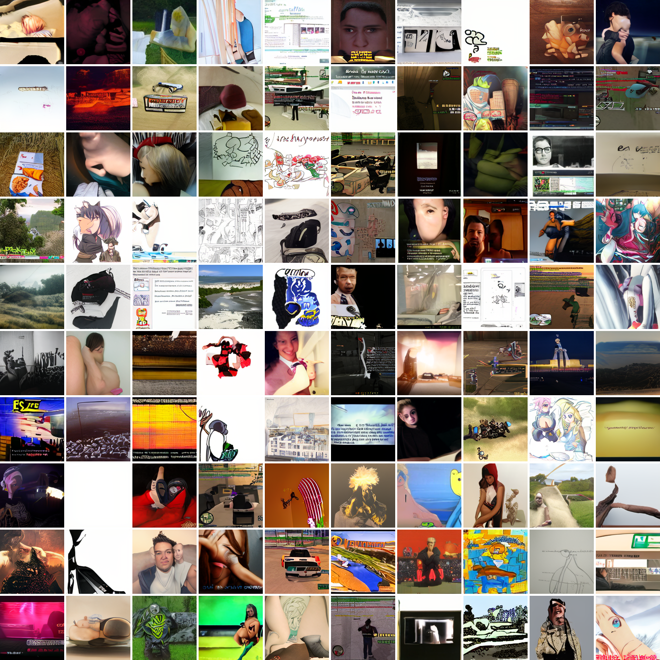
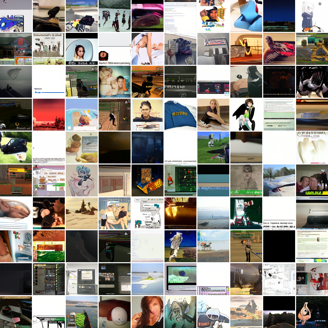
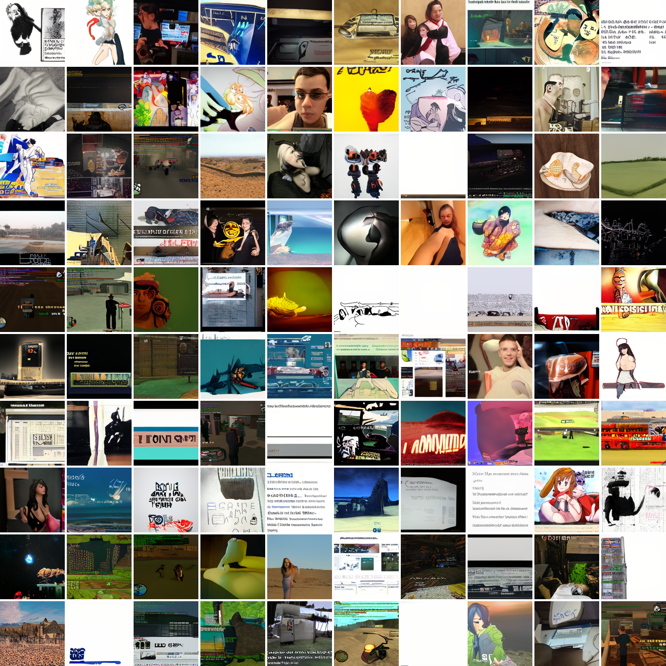
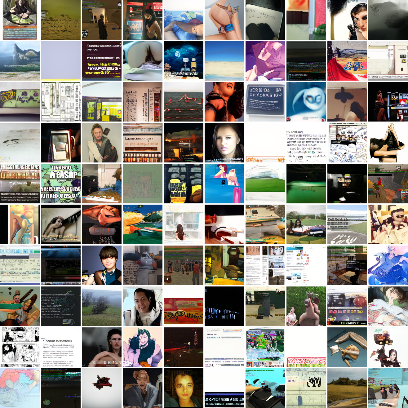
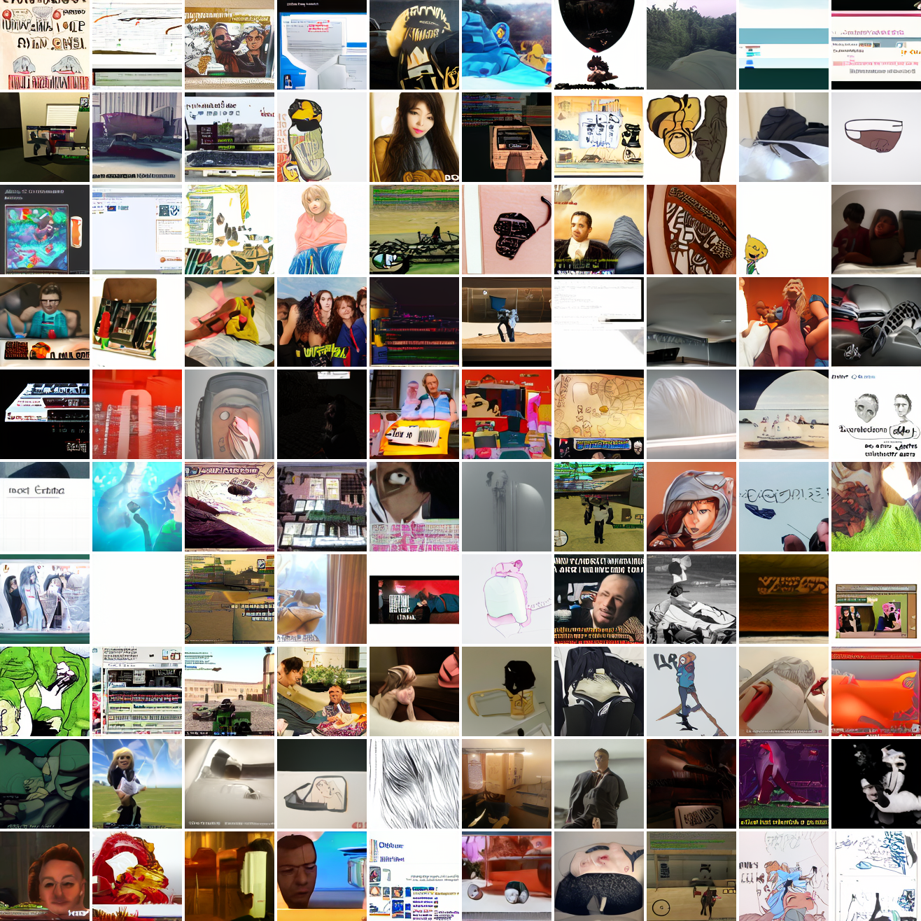
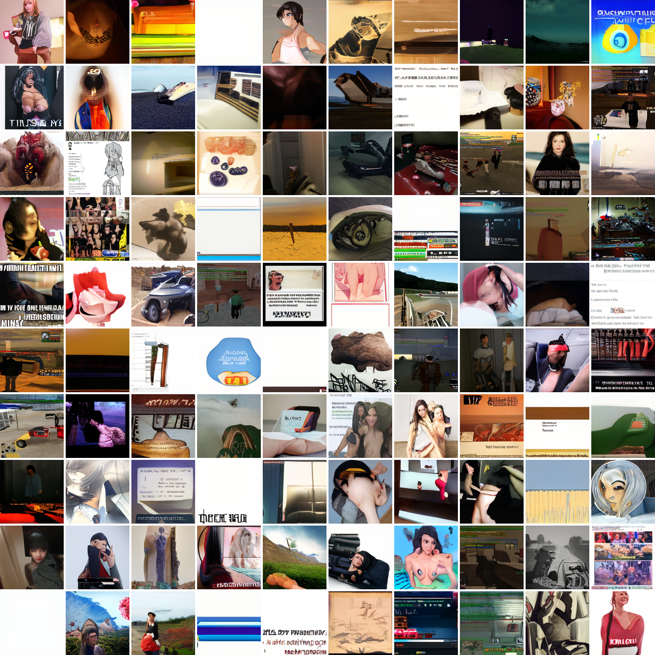
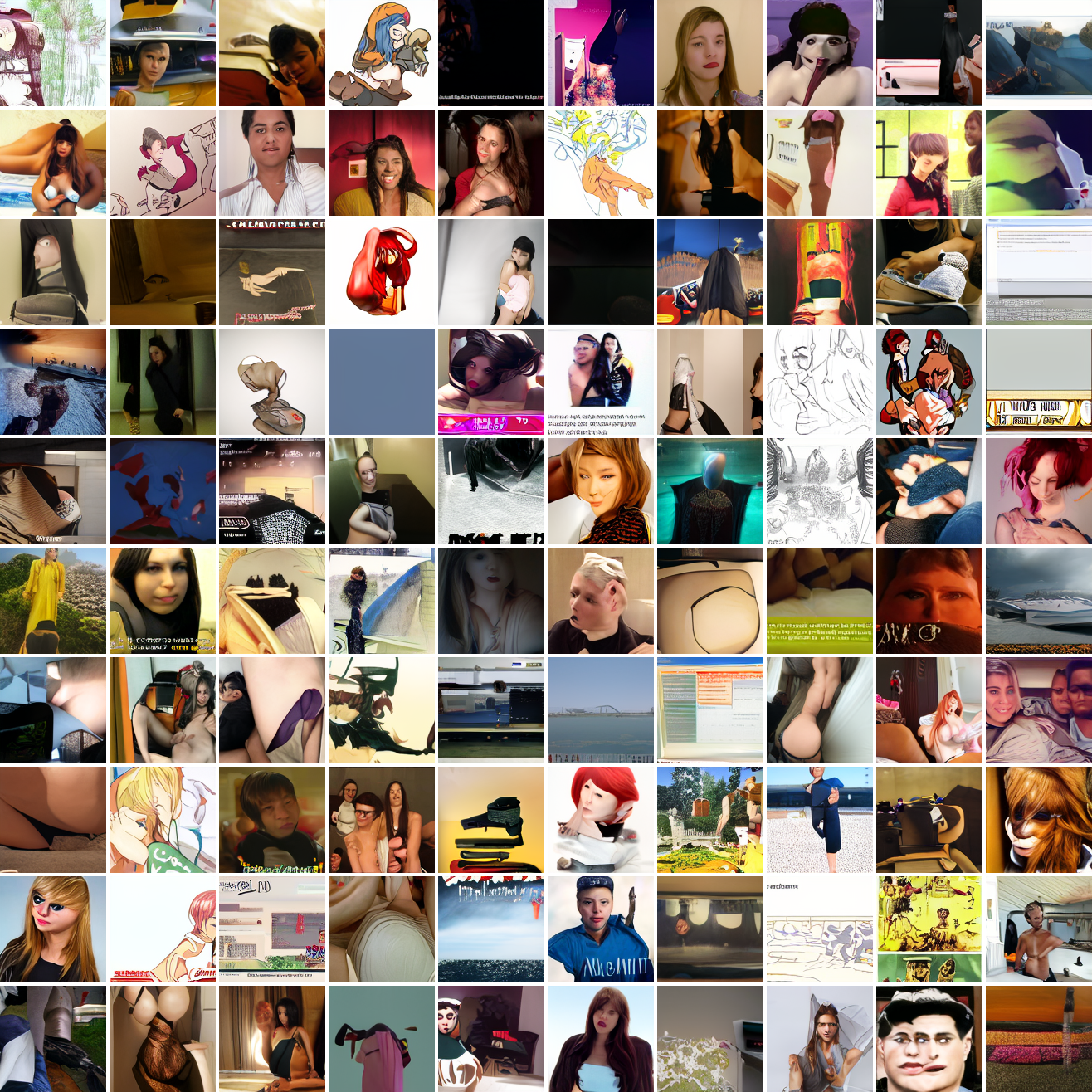
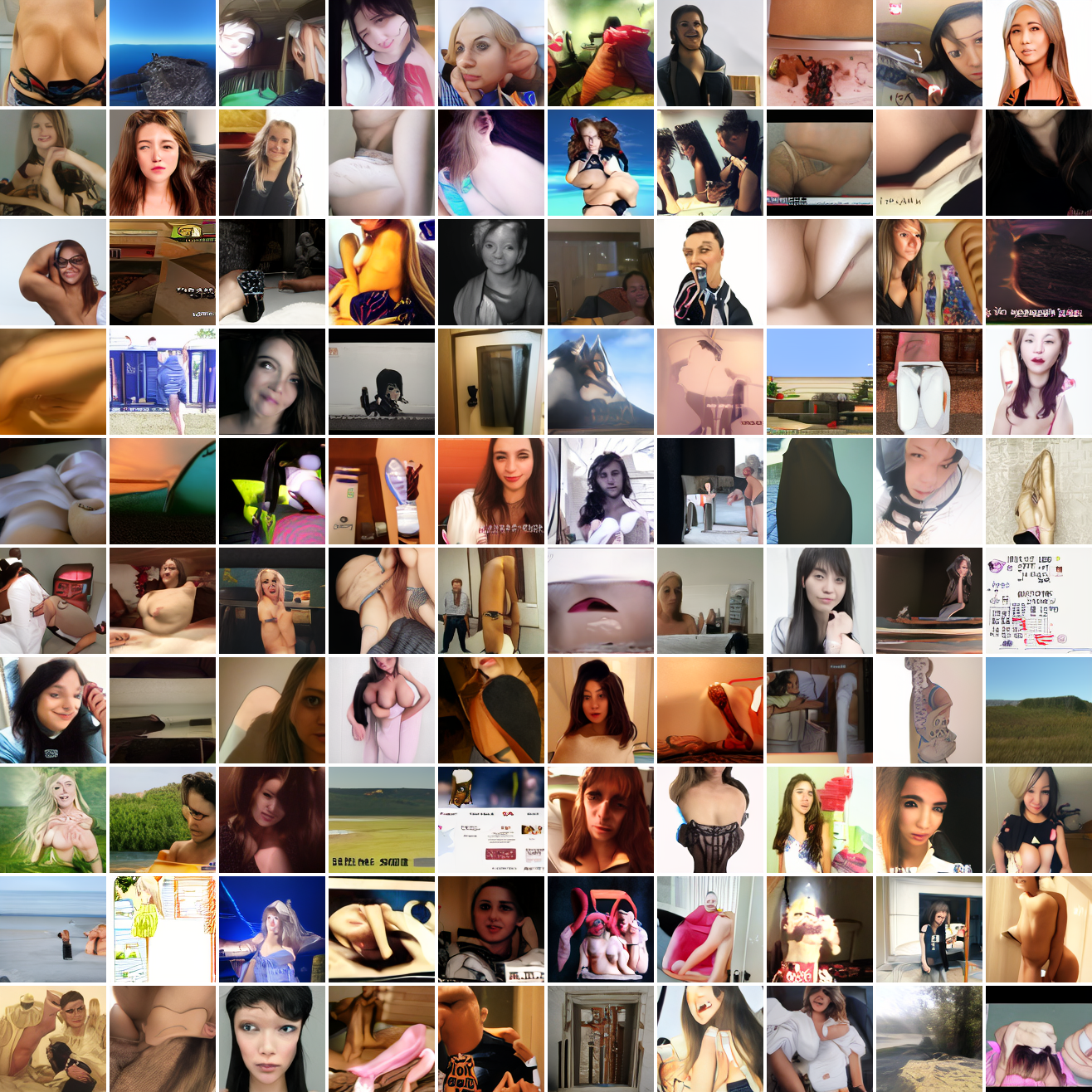
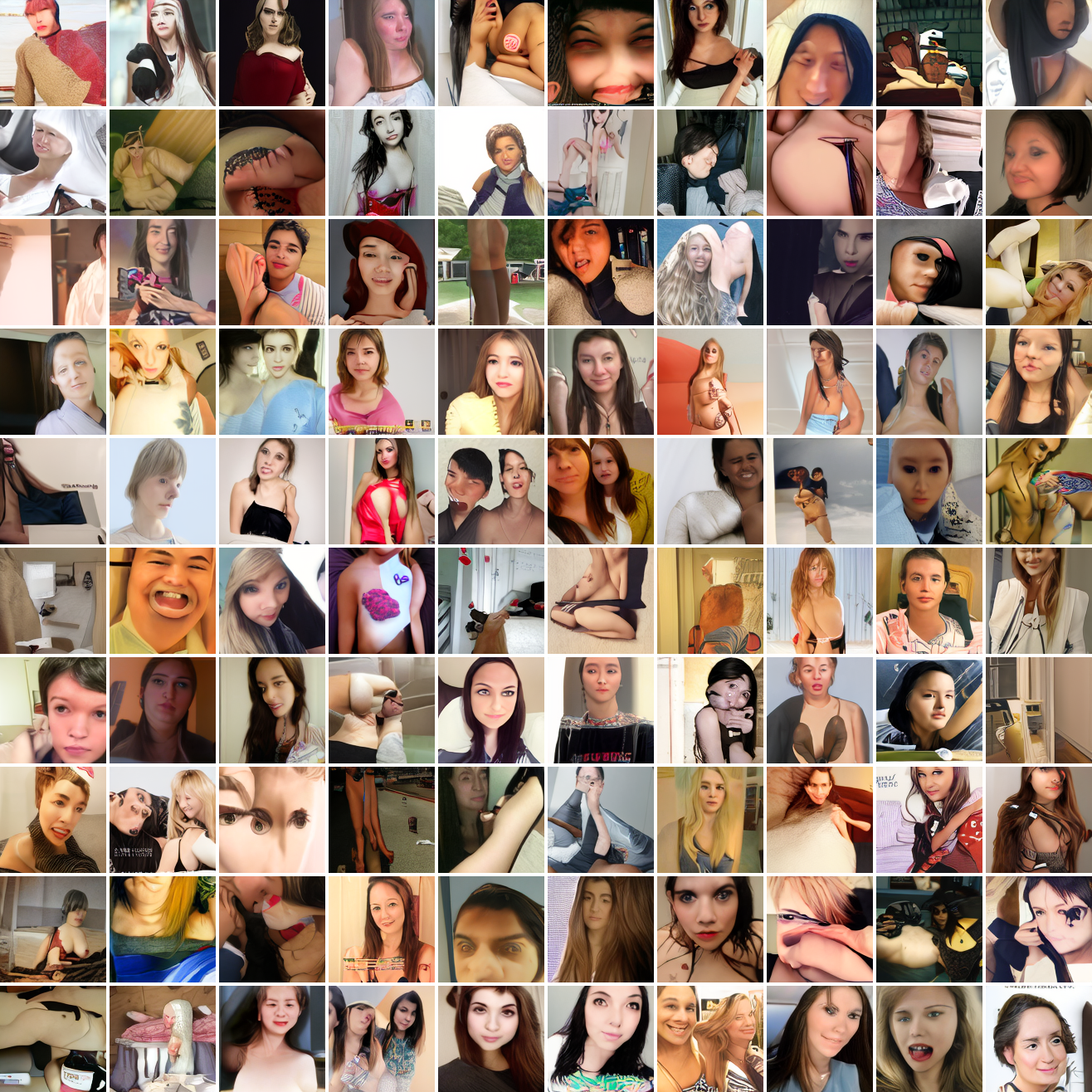
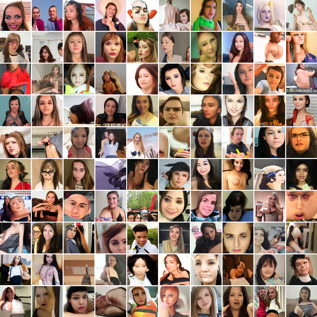
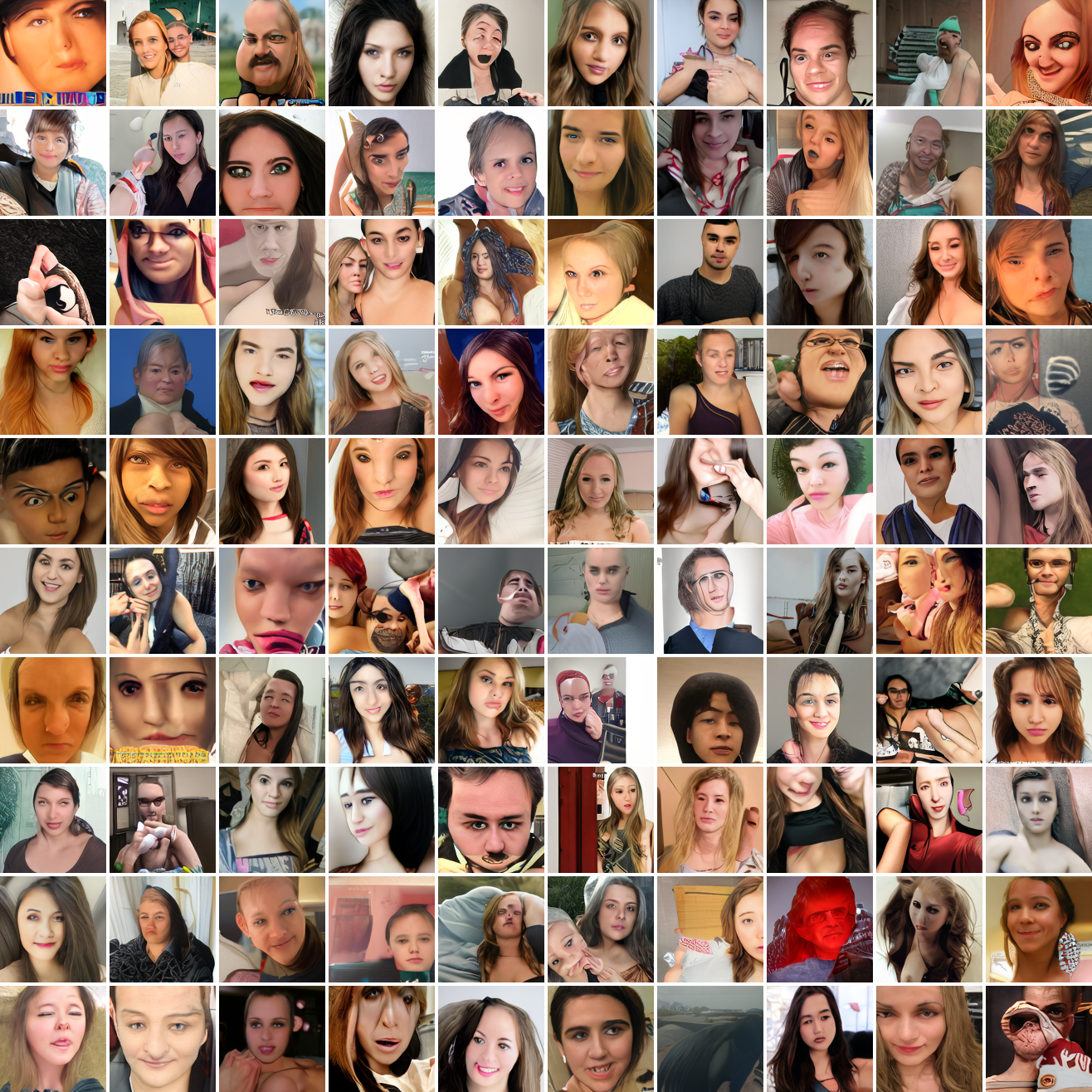
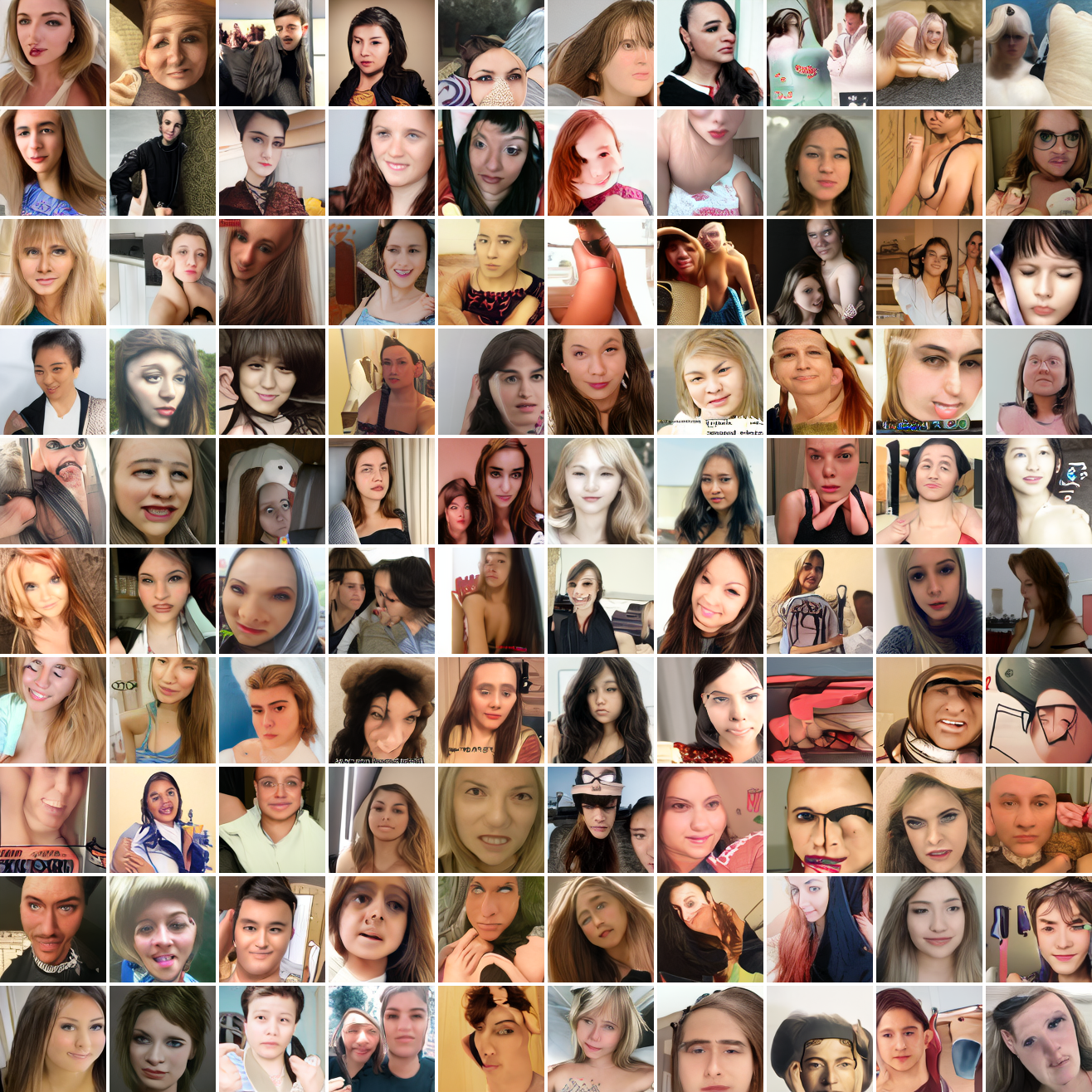
At max cosine distance 2.0, the samples are highly diverse and largely incoherent. Of the images where you can actually tell what it is, there are screenshots of websites, faces and figures, screenshots of video games, screenshots of GTA, and landscapes. This pattern continues up until around 0.5, when faces become the most common type of image. As the size of the cap continues to get smaller, the images get more consistent, with the pose and positioning of the faces becoming more homogenous.
Now let’s see a similar series of images conditioned on the embedding of a GTA screenshot.
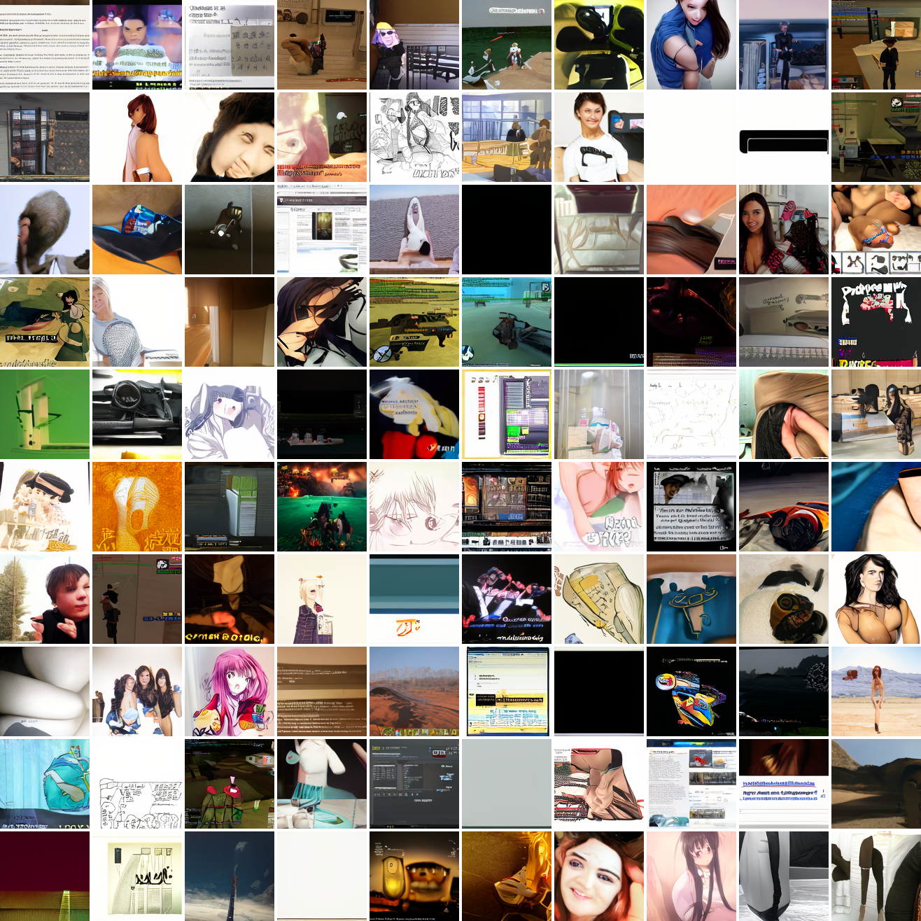
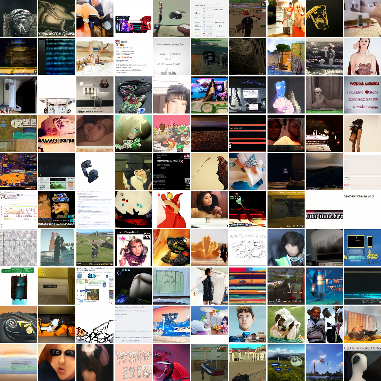
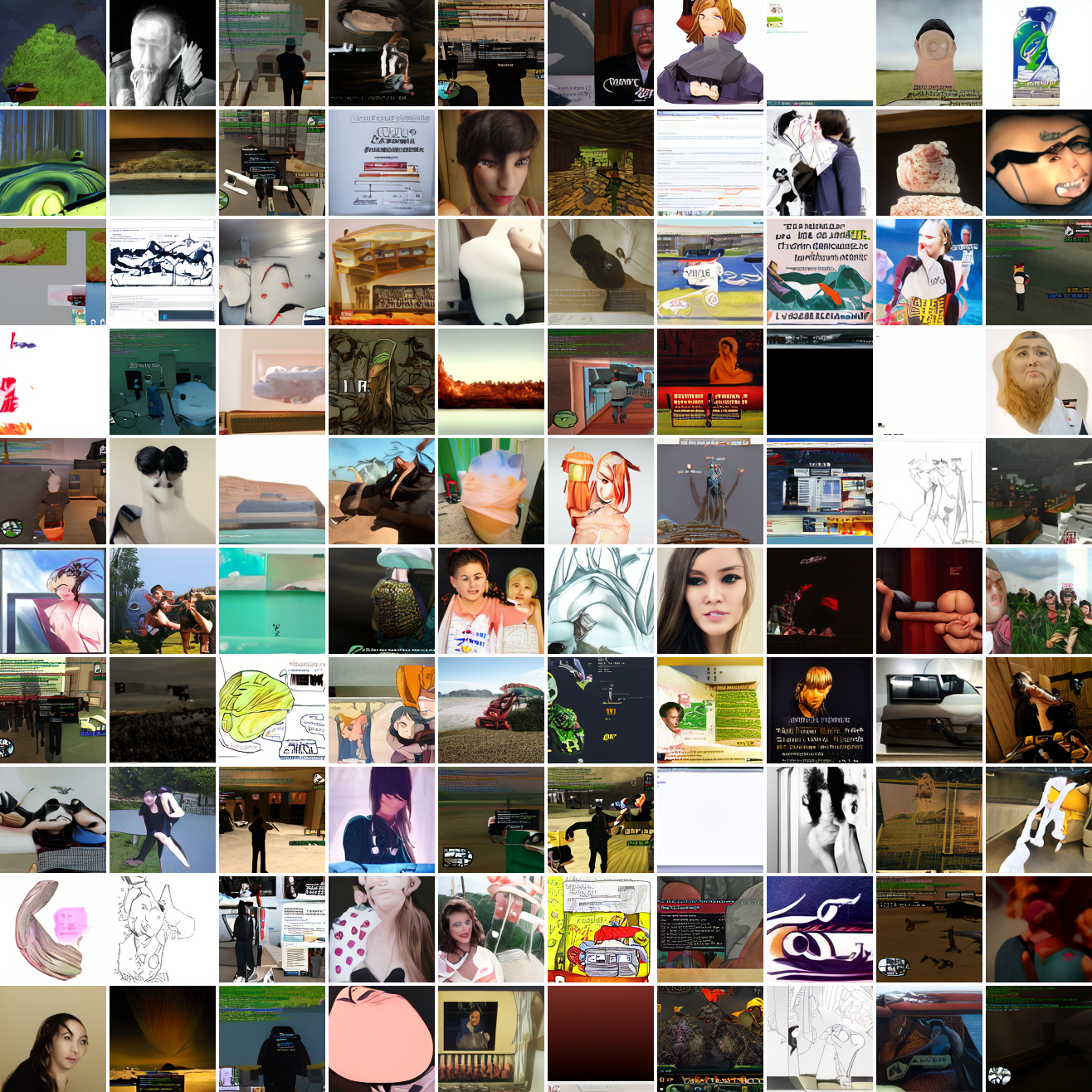
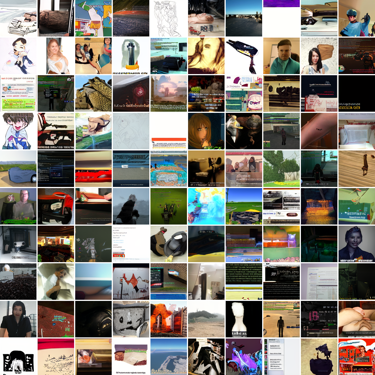
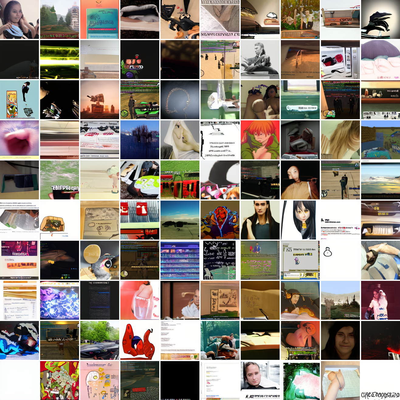
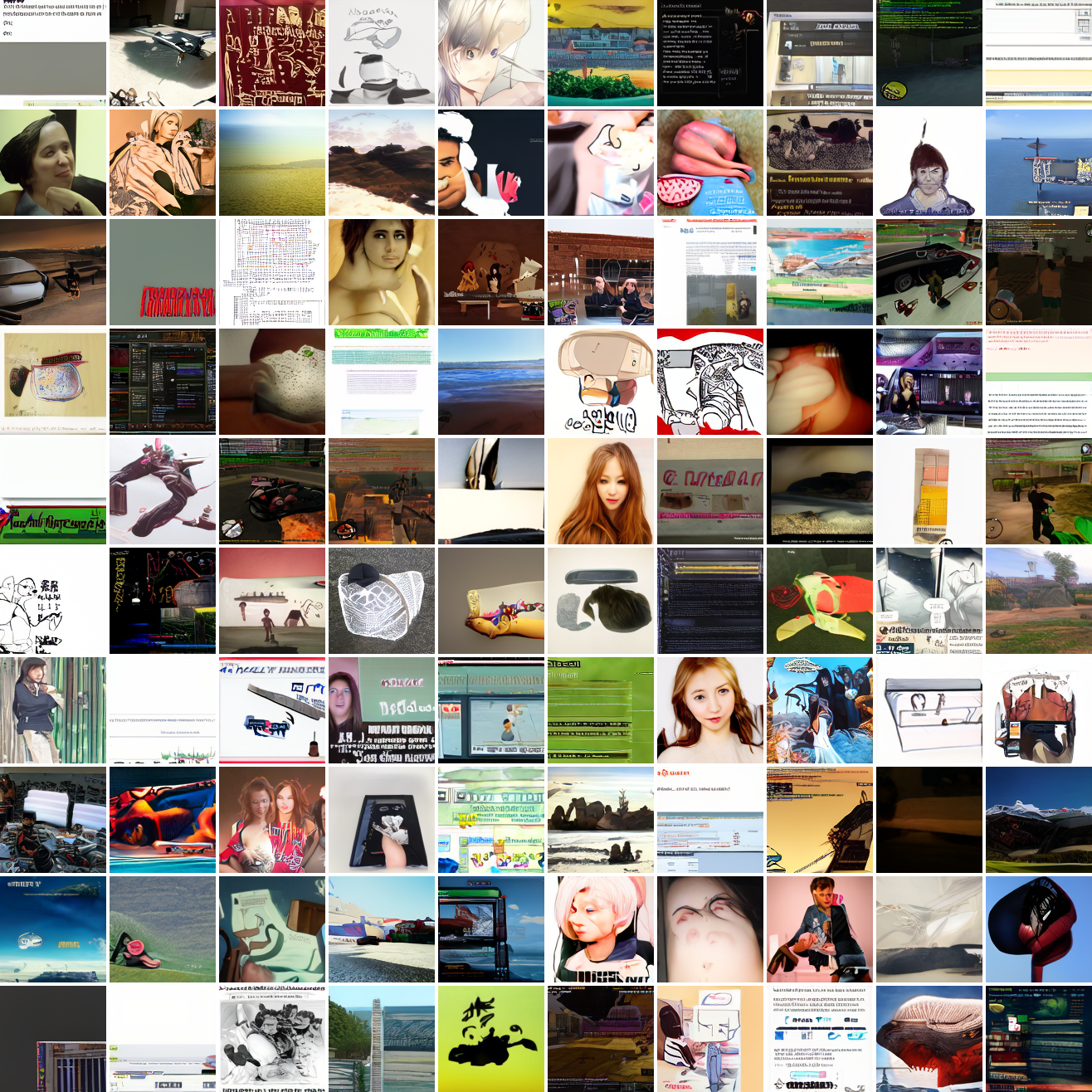
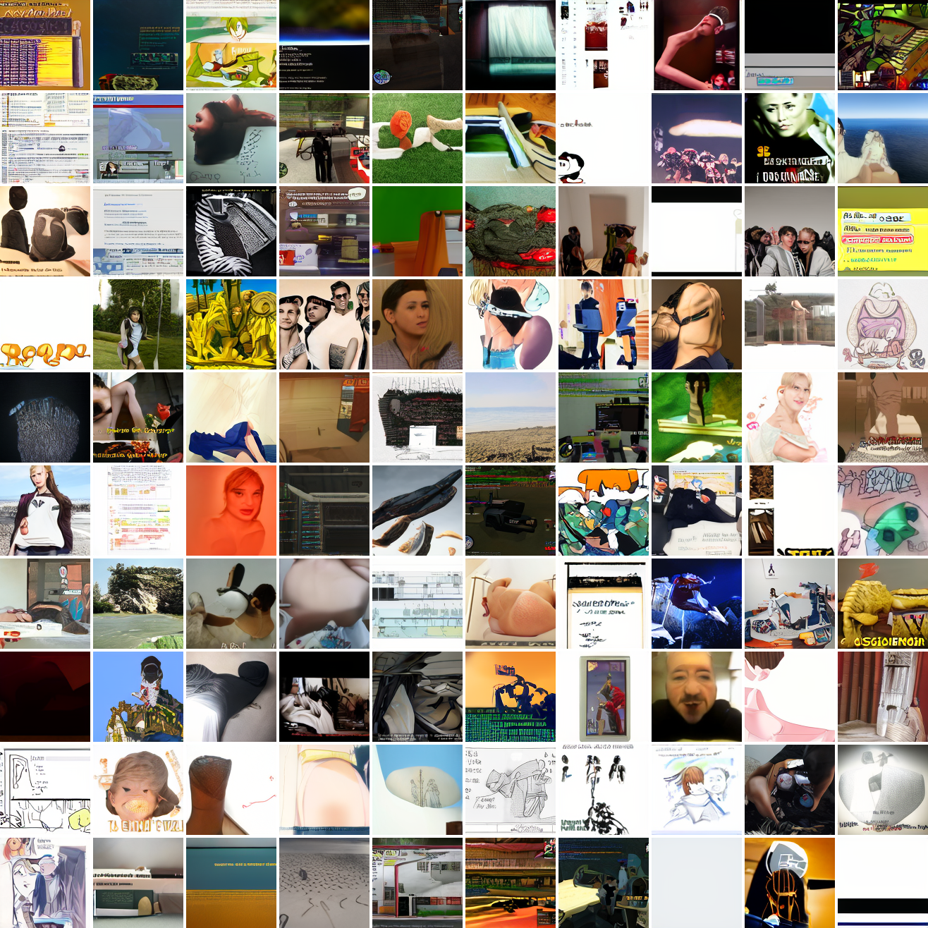
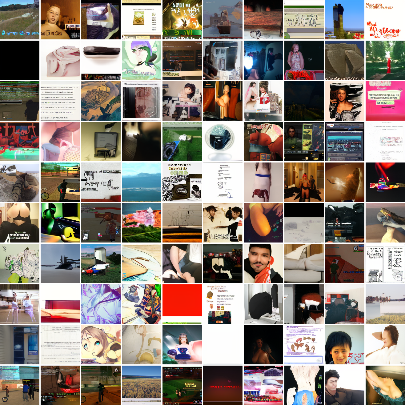
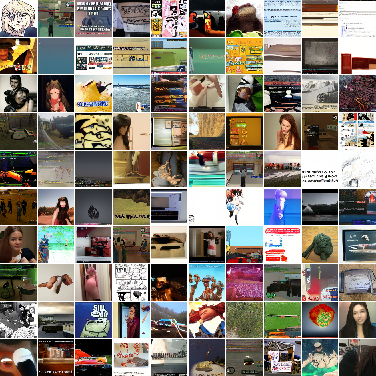
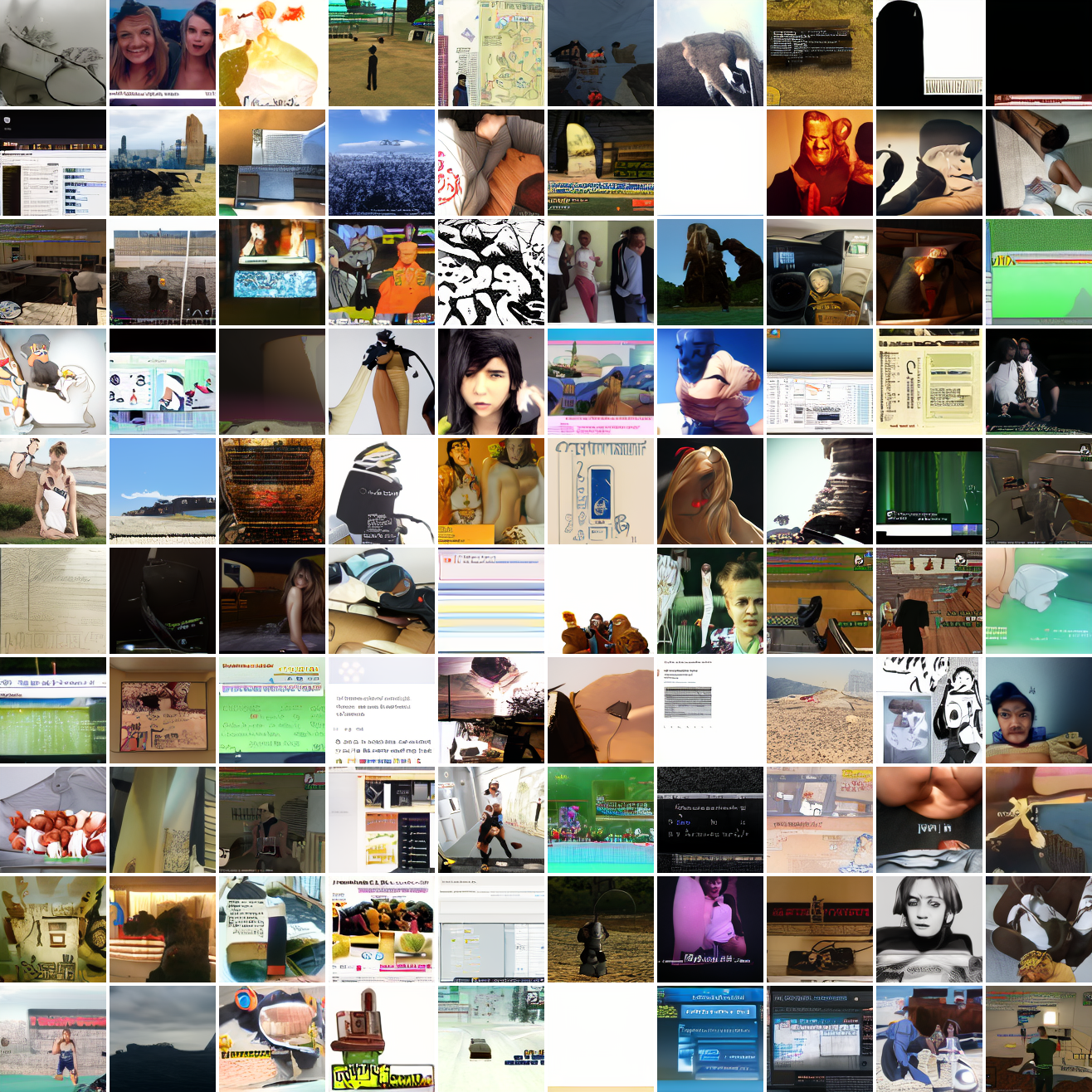
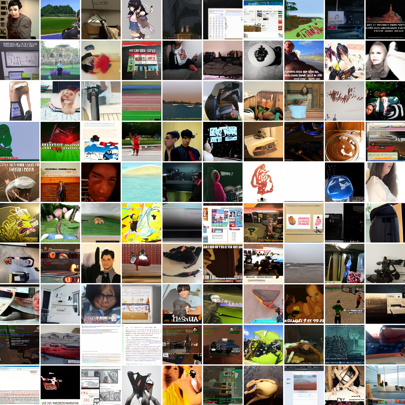
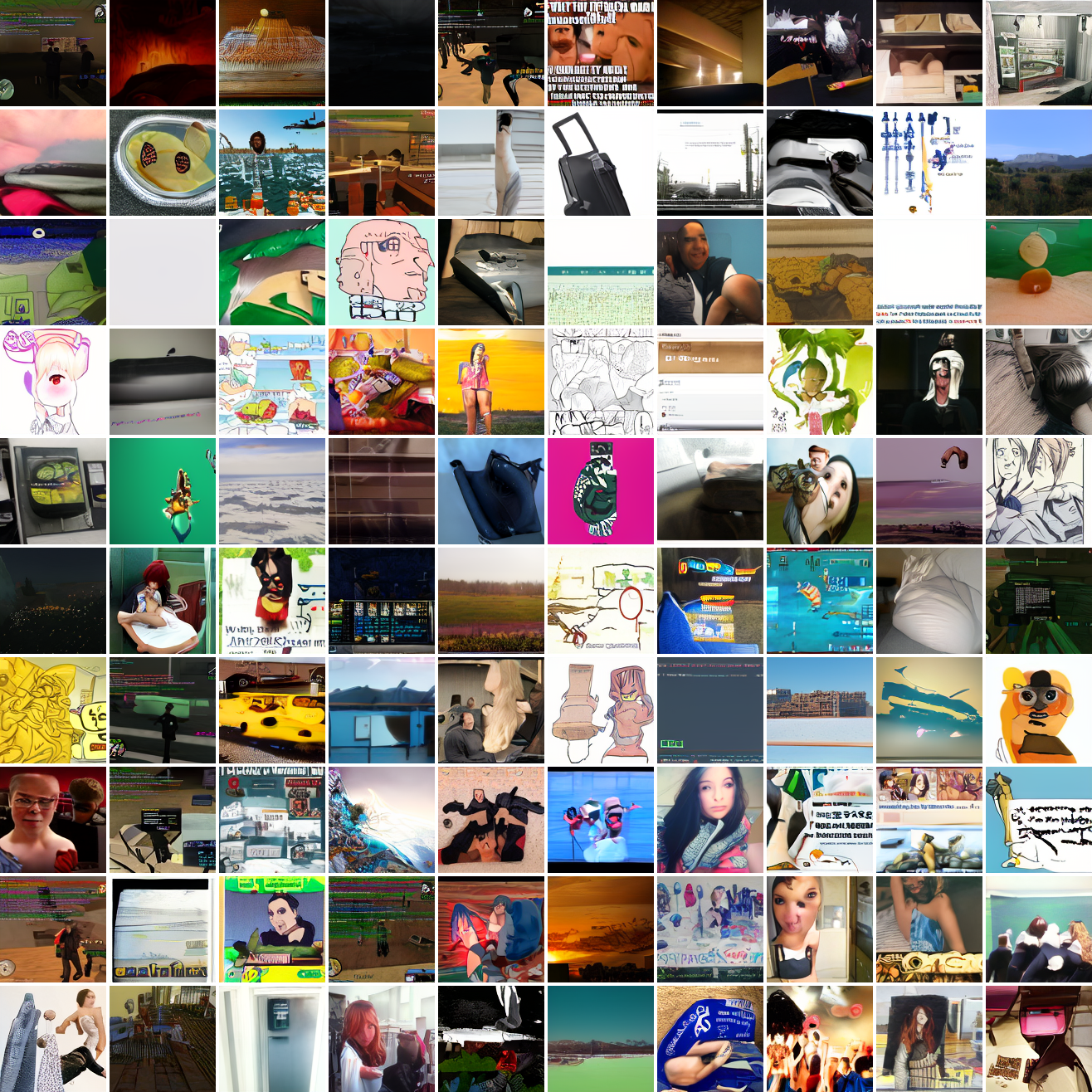
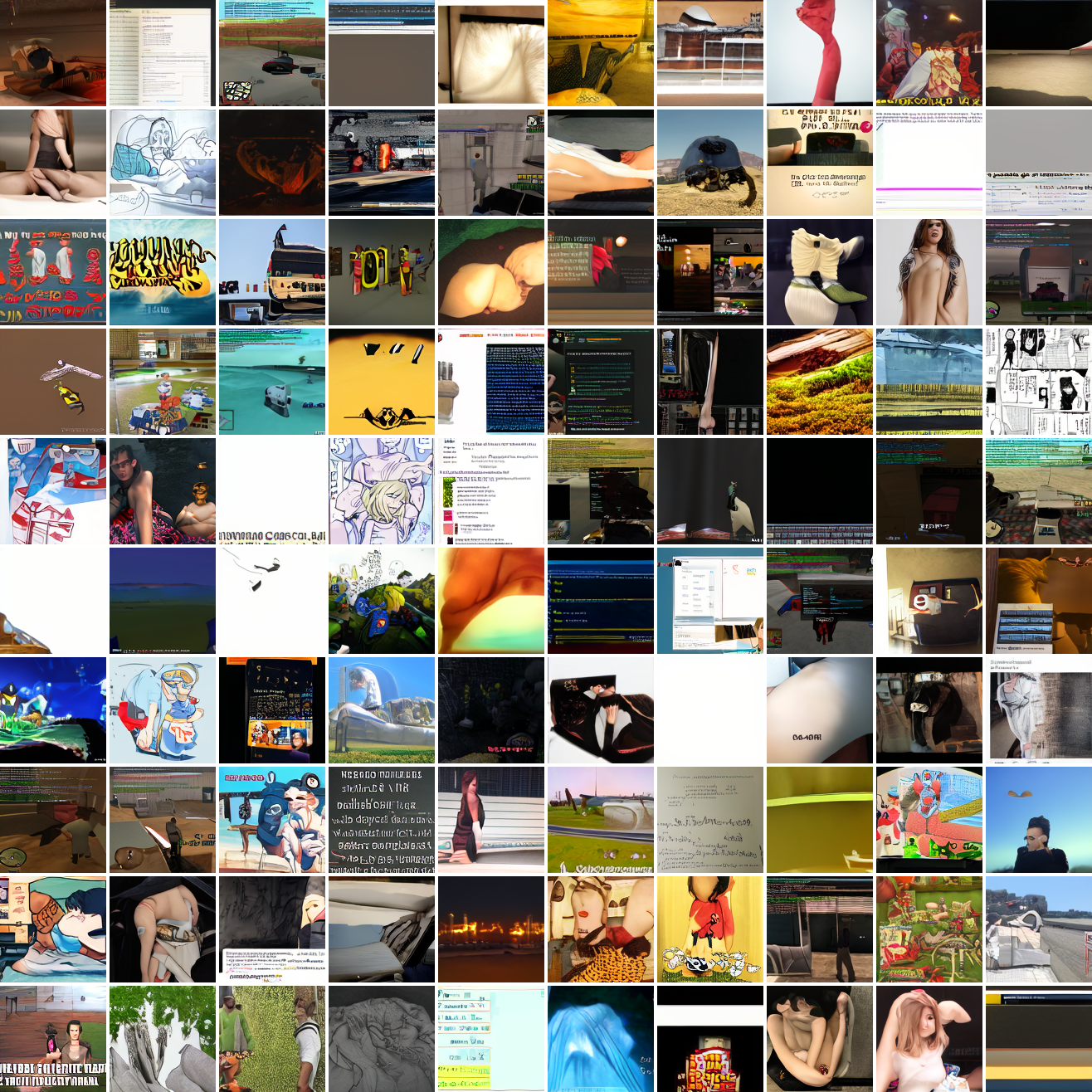
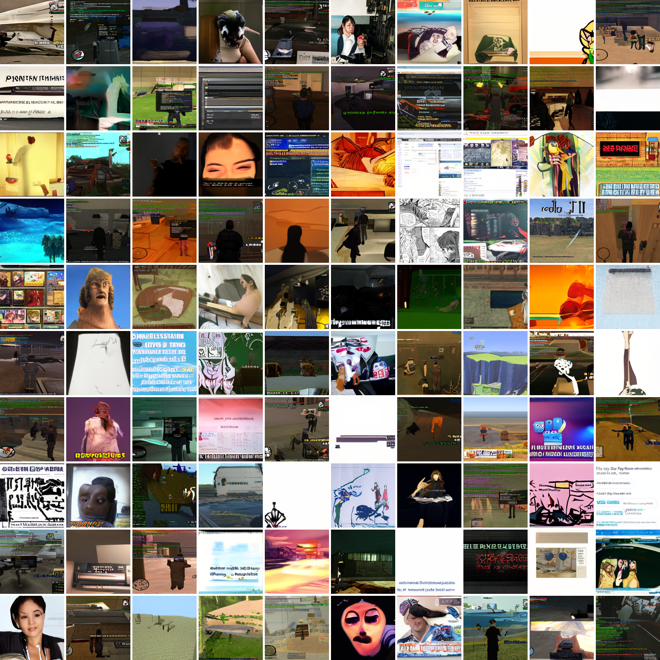
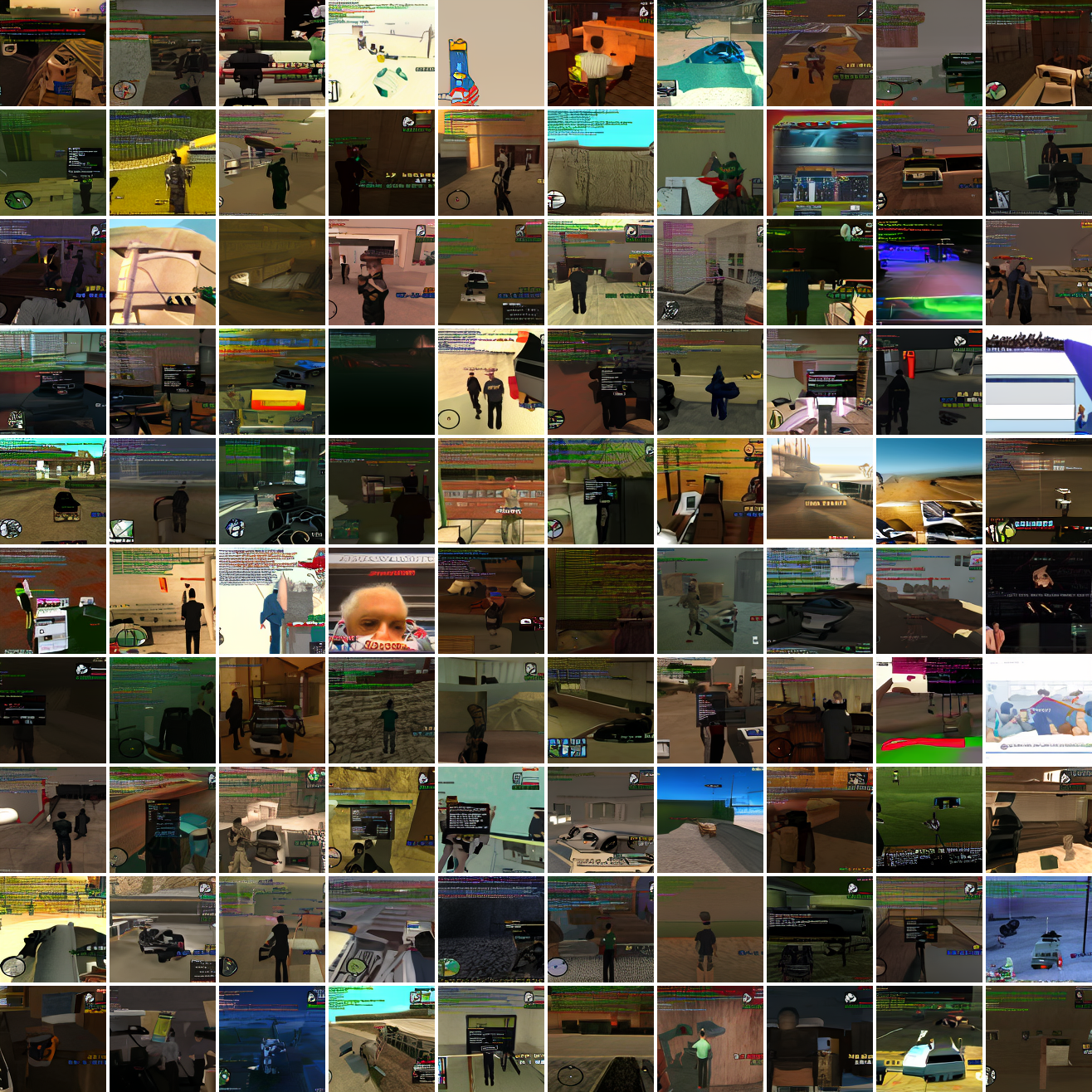
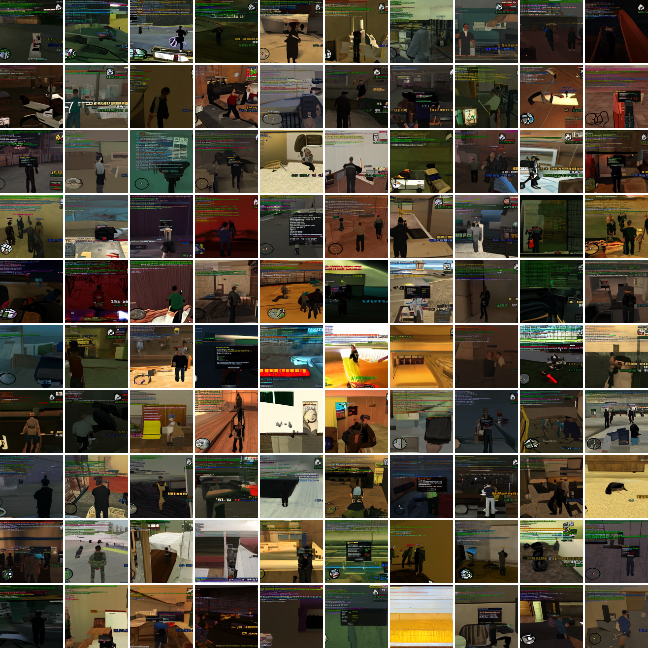
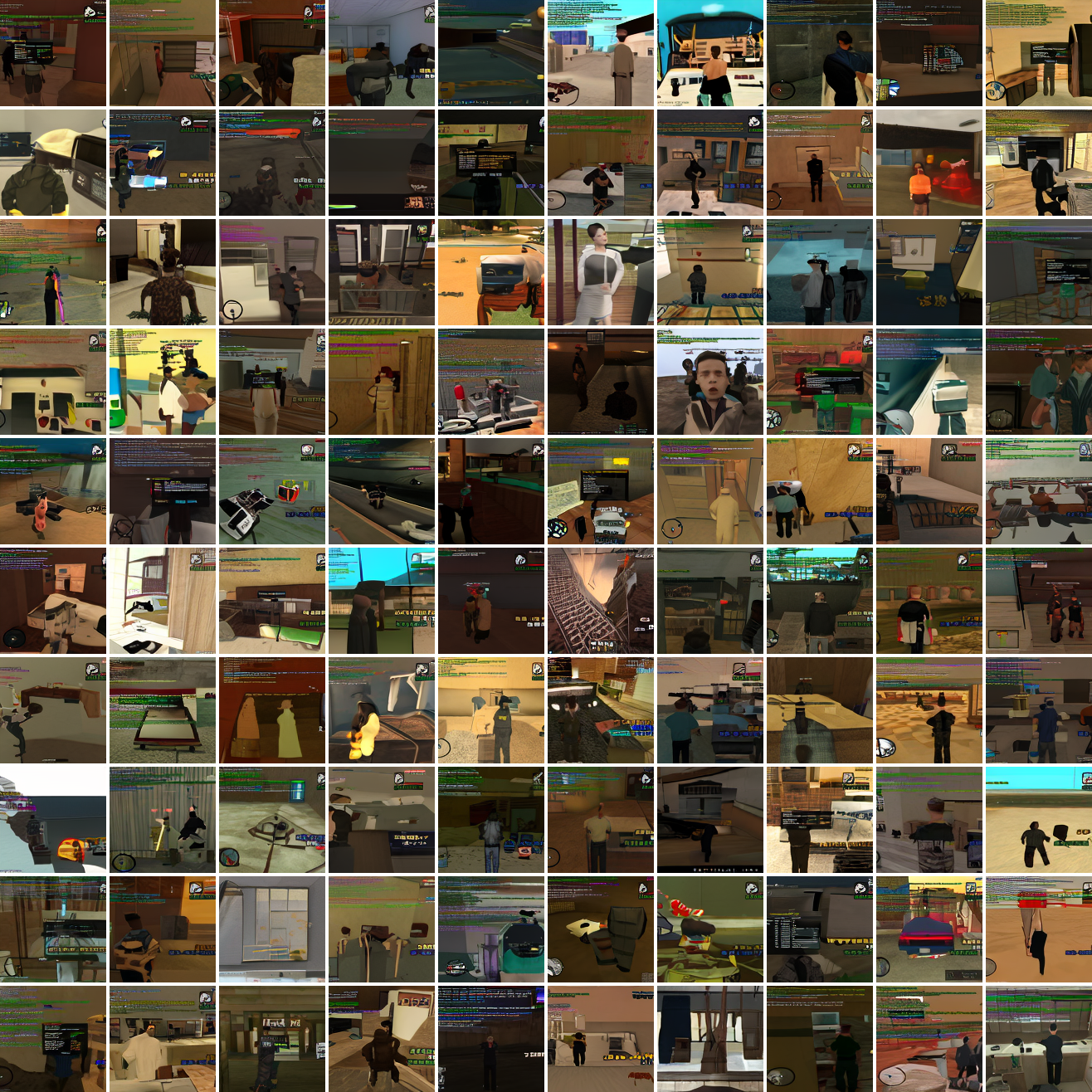
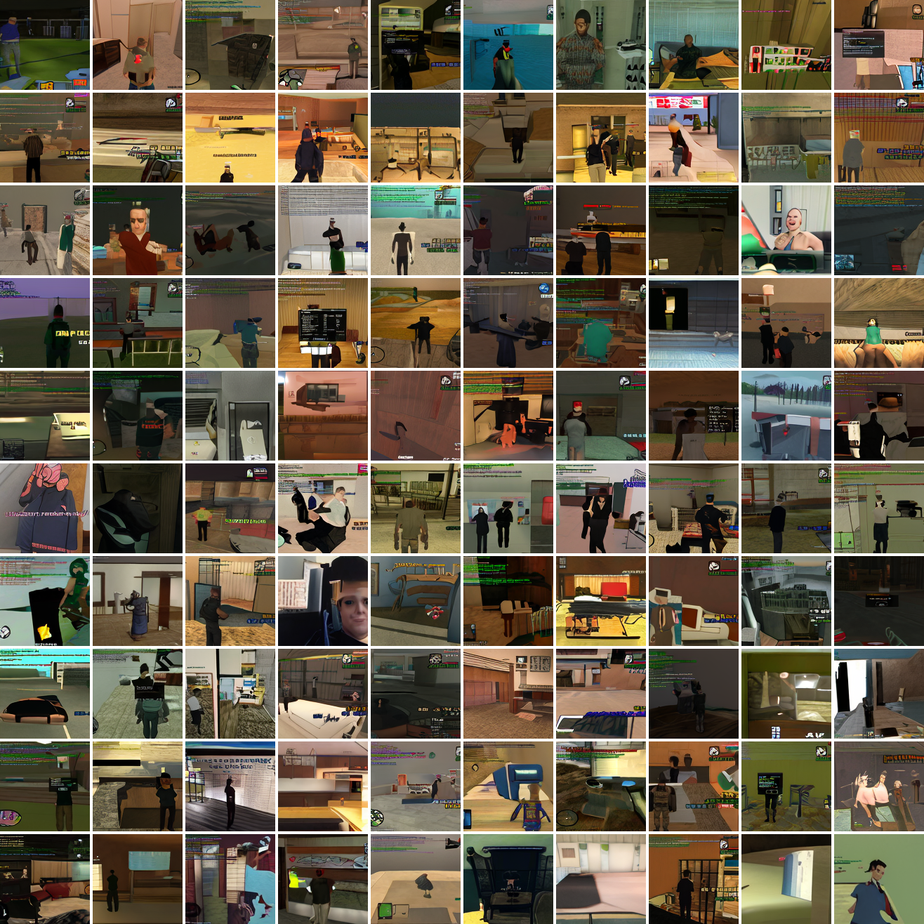
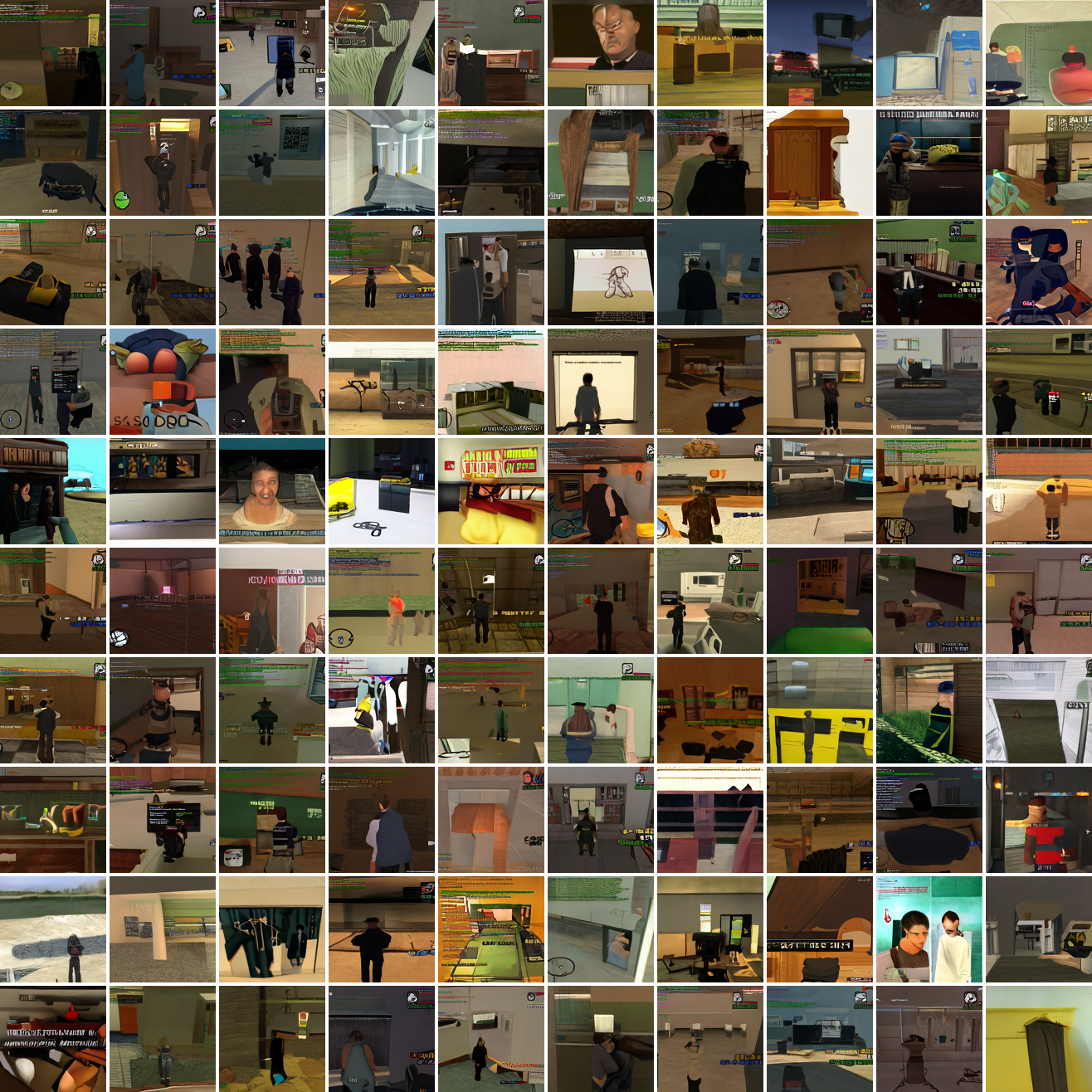
This is about what you’d expect from a model like this, but in a good model you’d start seeing mostly faces or mostly screenshot type things around 0.9 or 0.8.
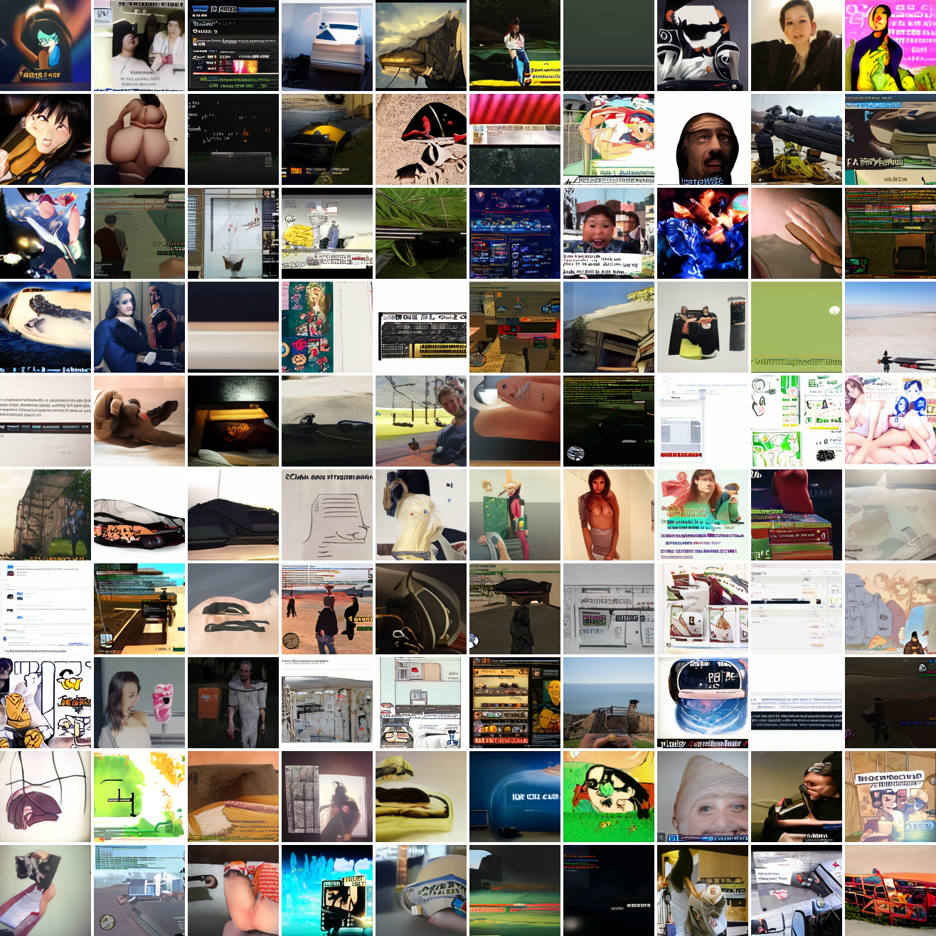
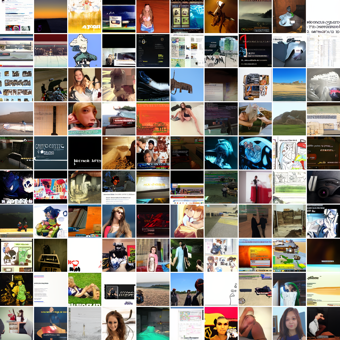
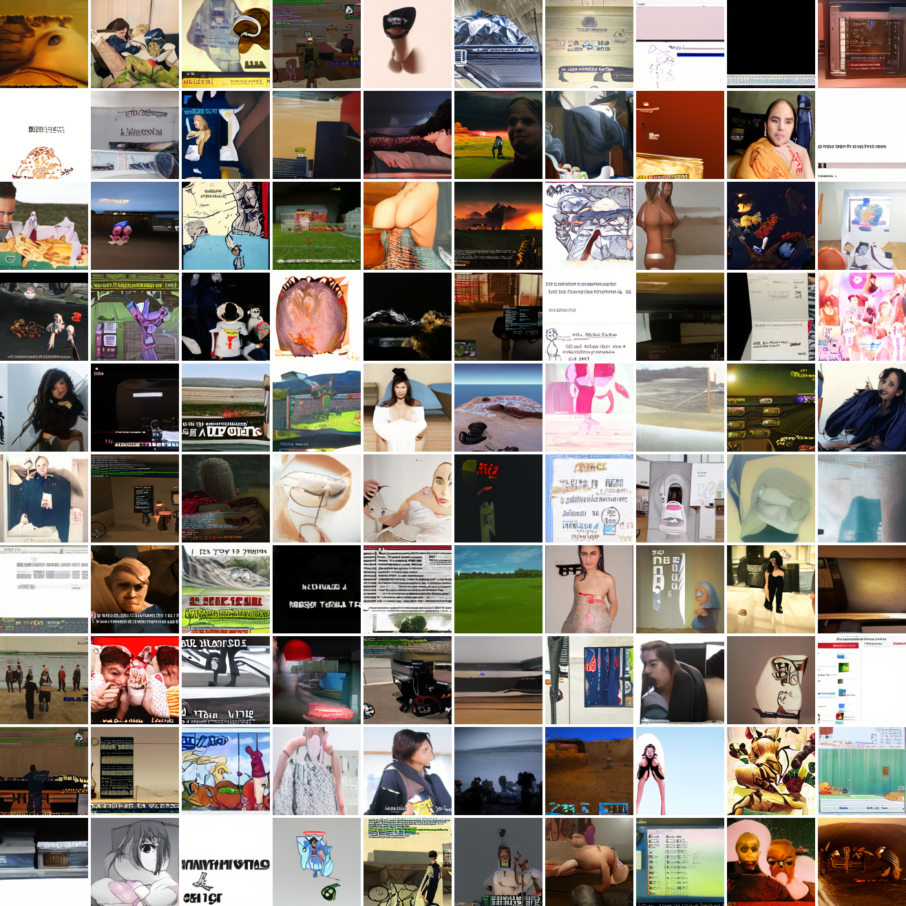
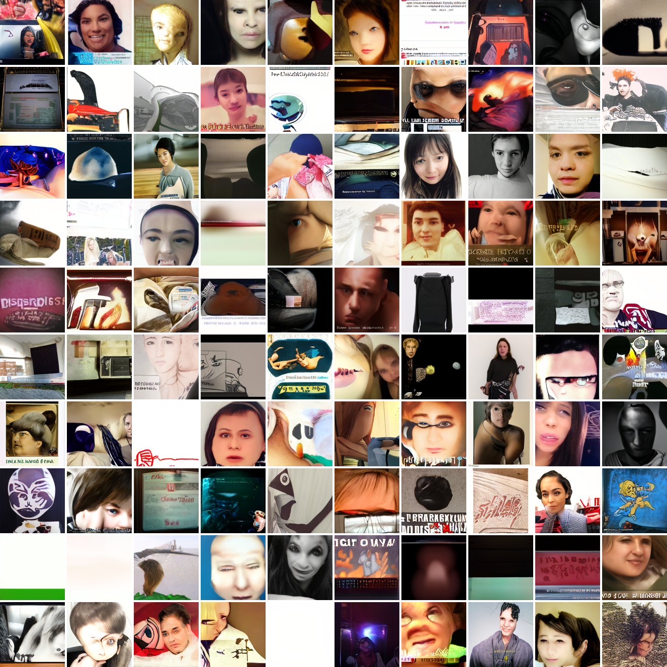
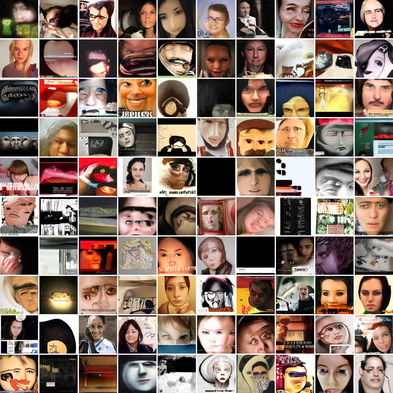
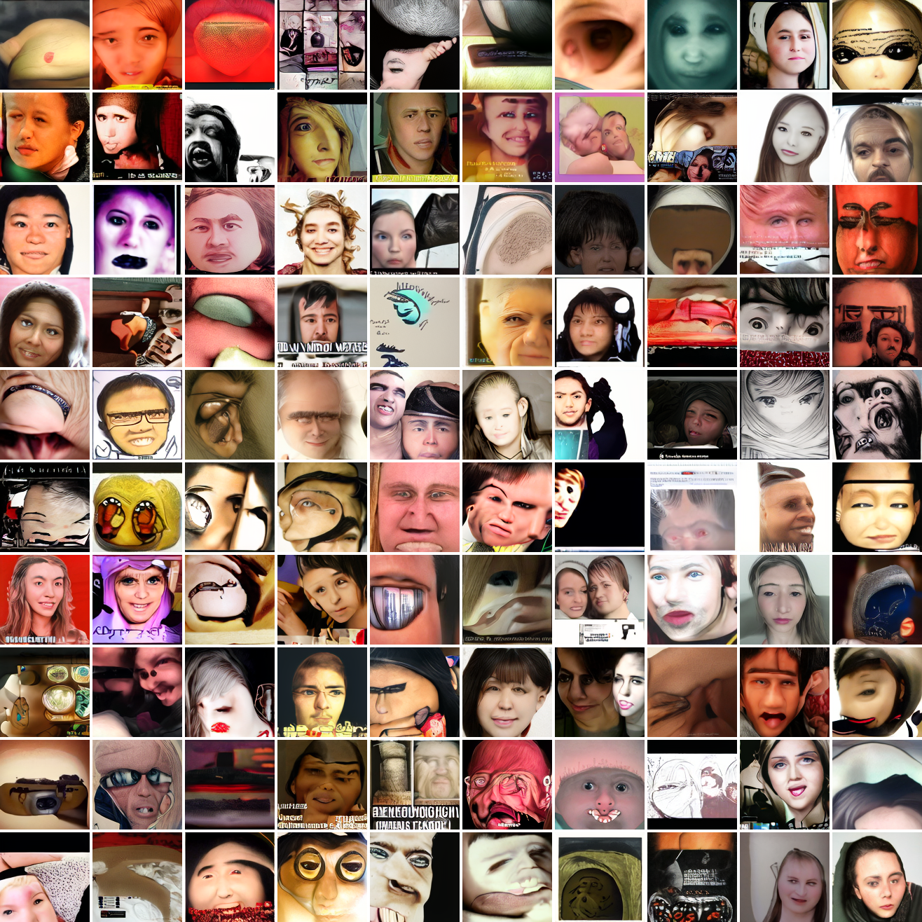
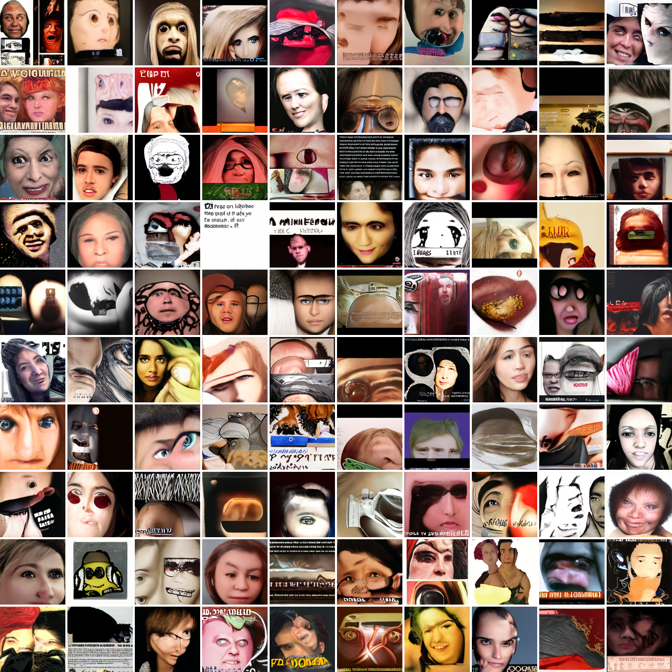
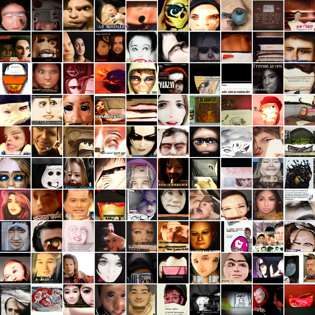
Let’s try the text prompts I used with the baseline model. Here’s “A woman’s face”:
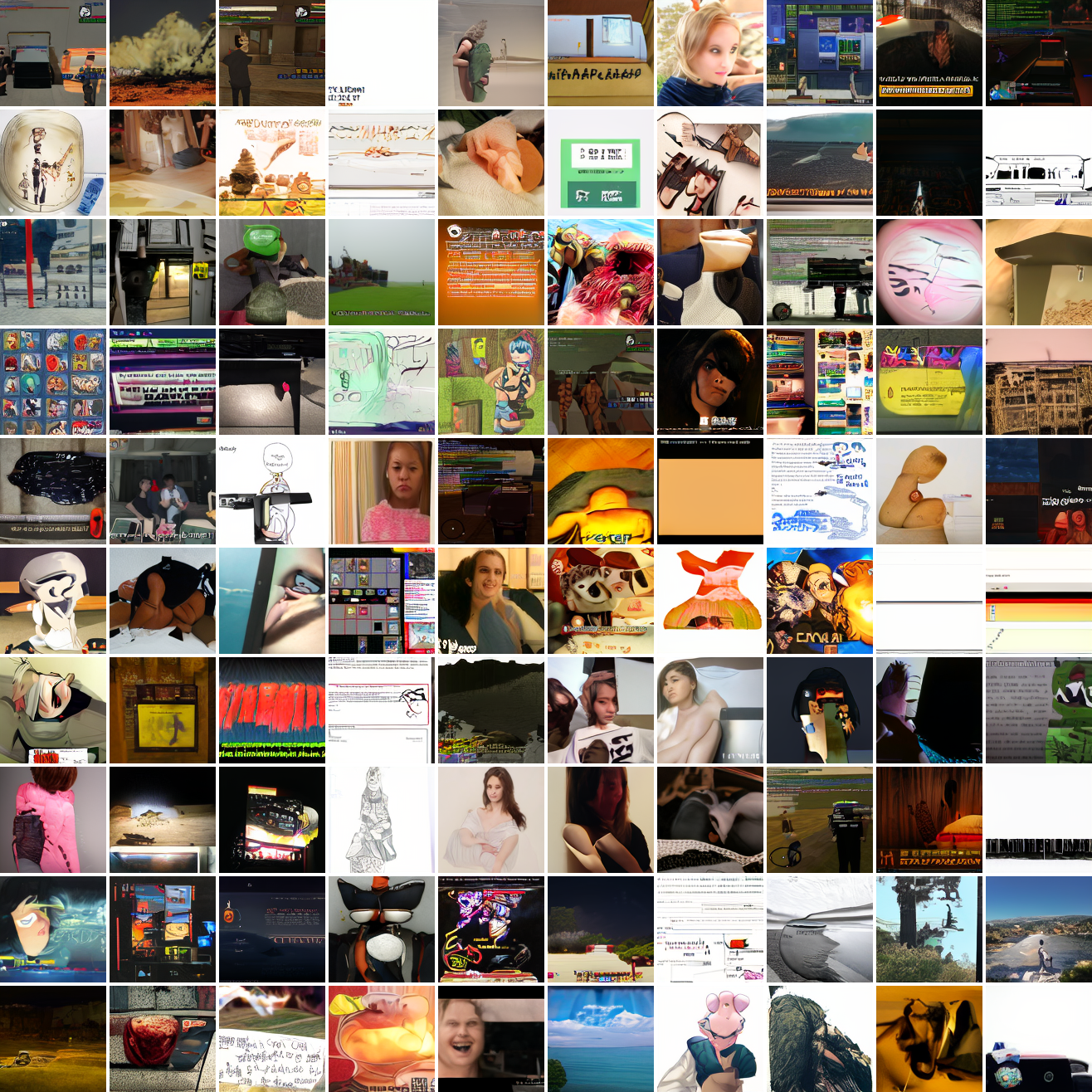
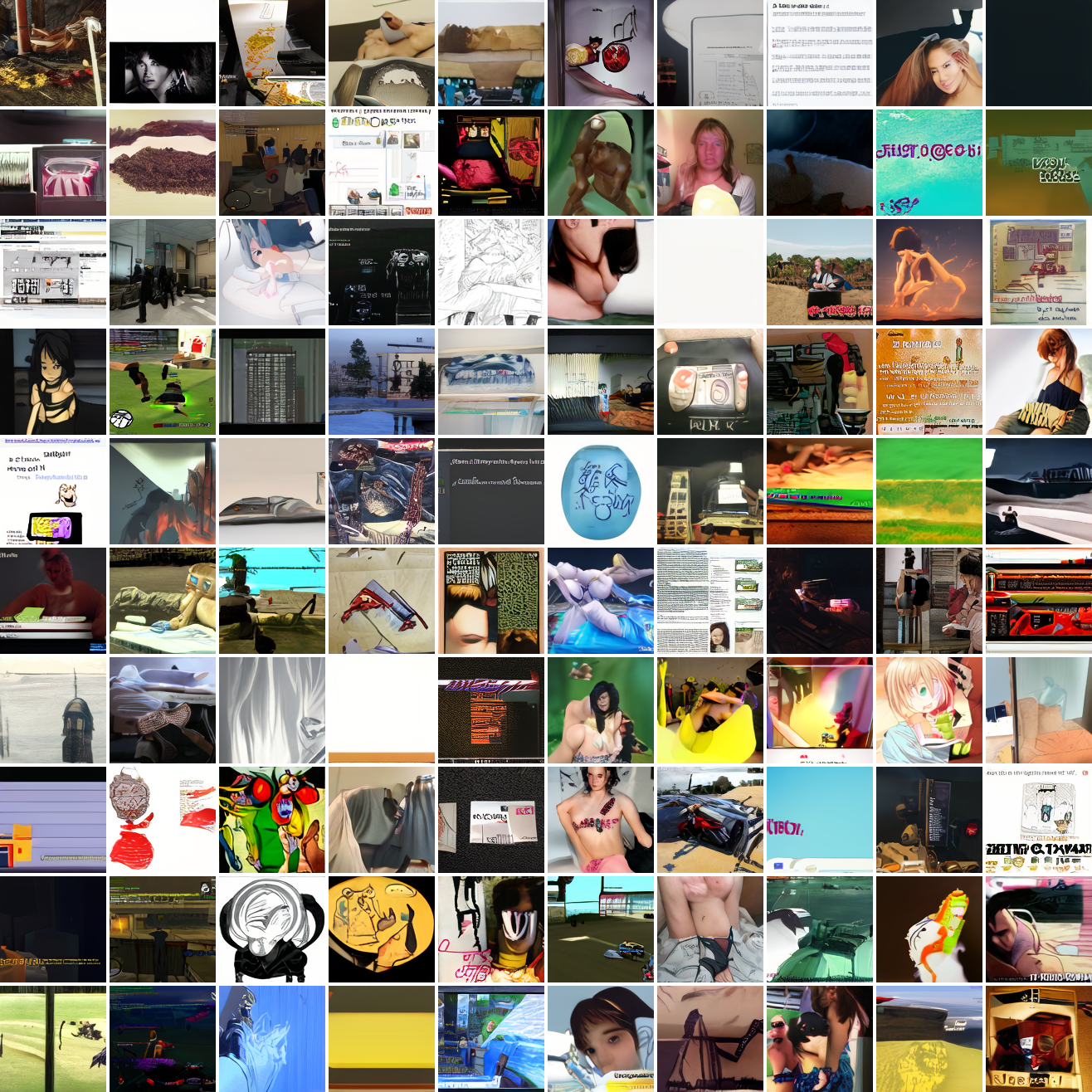
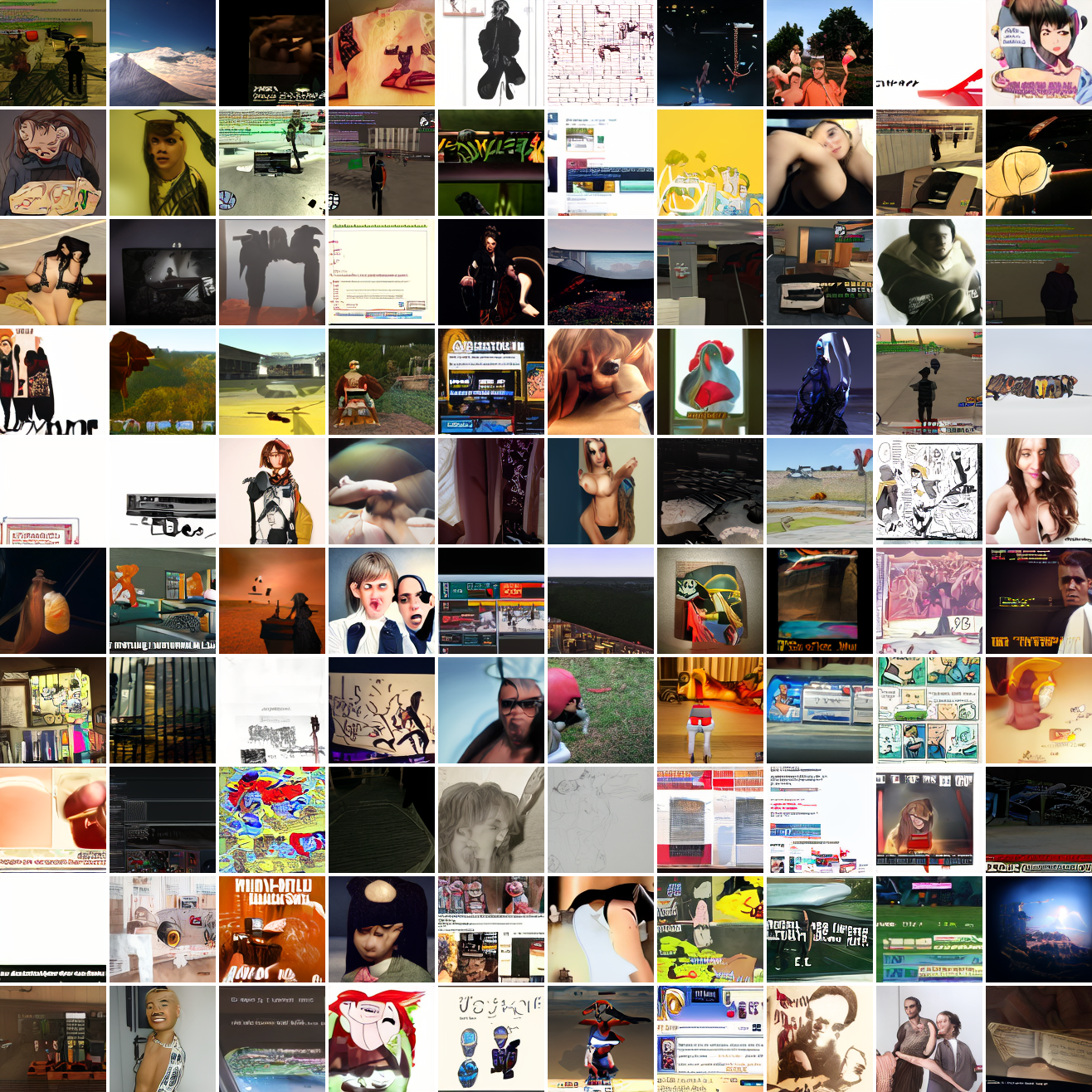
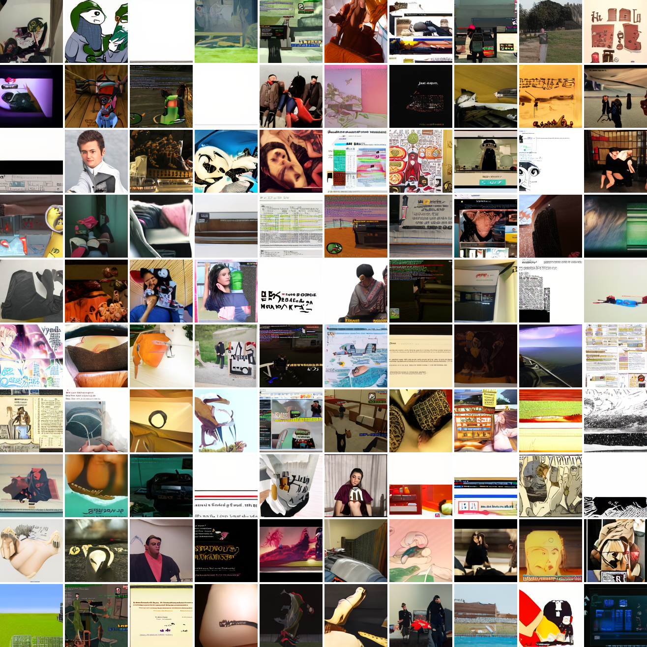
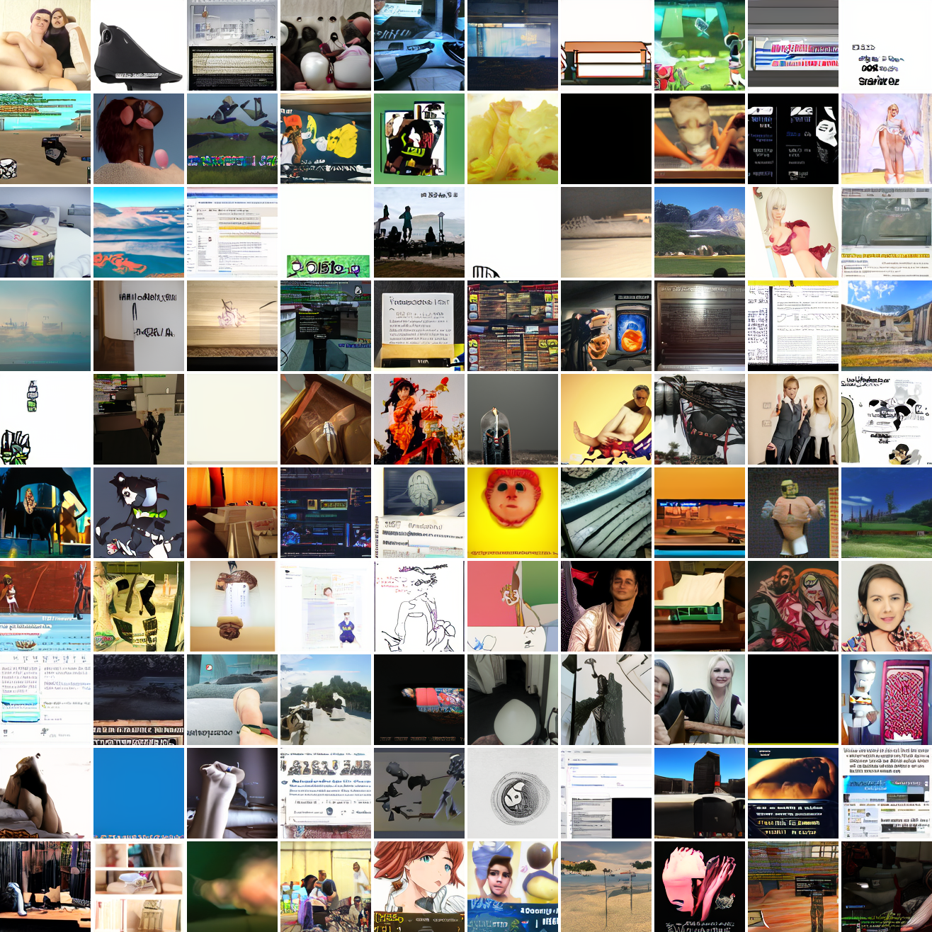
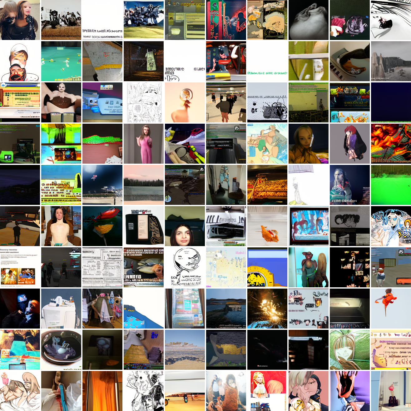
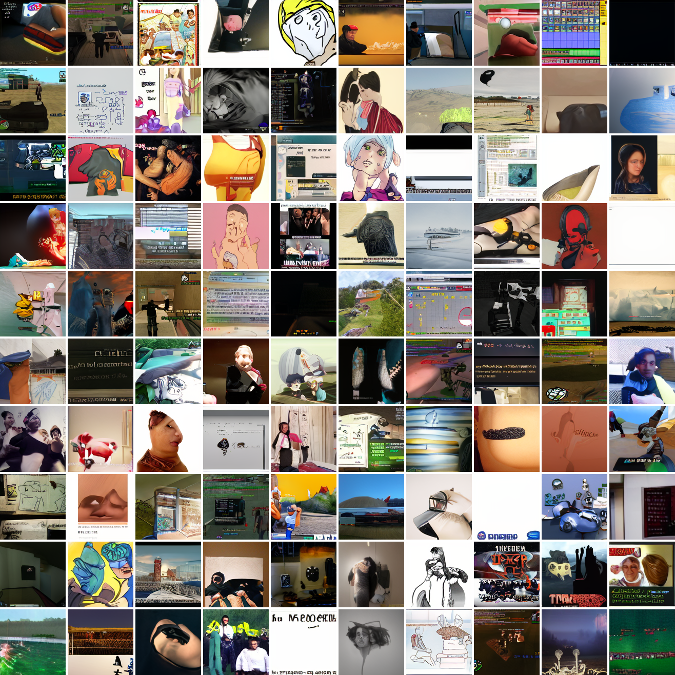
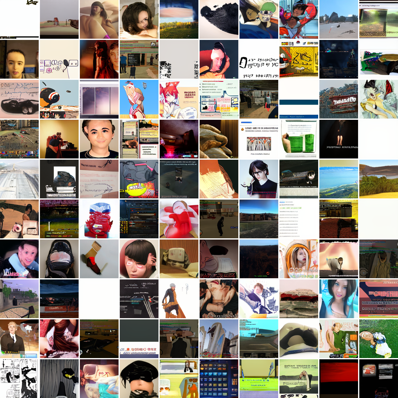
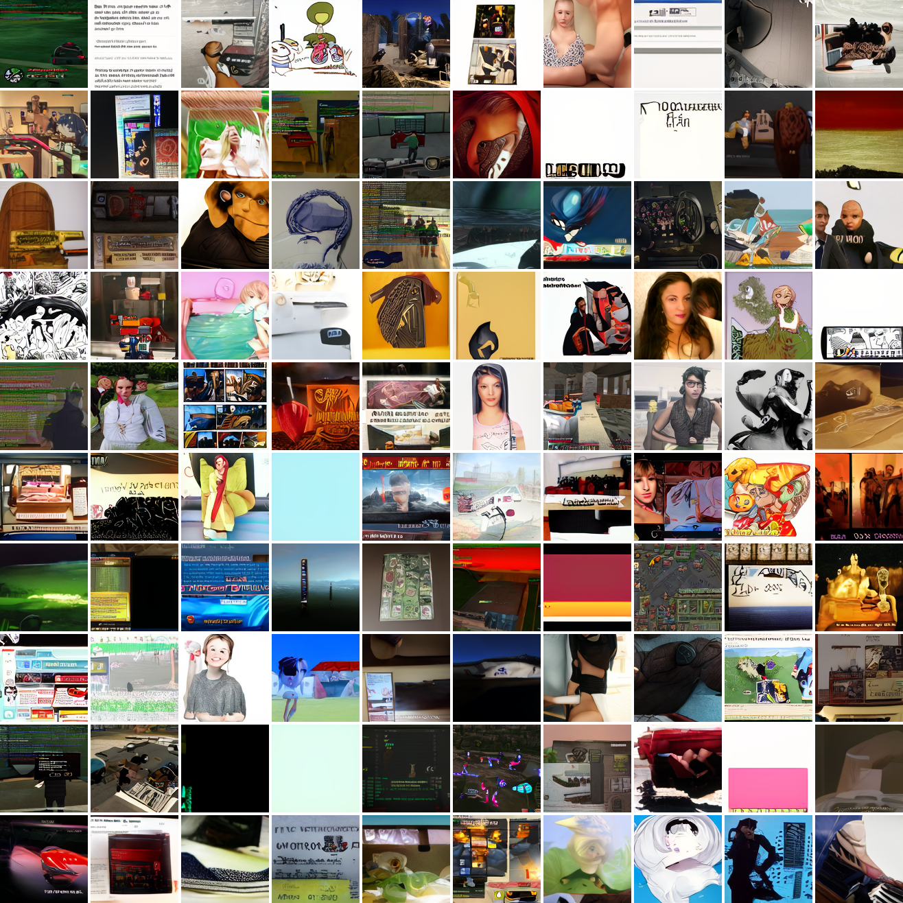
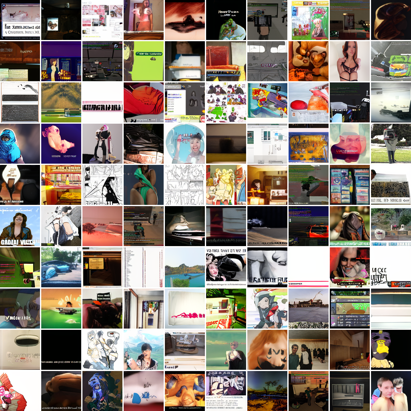
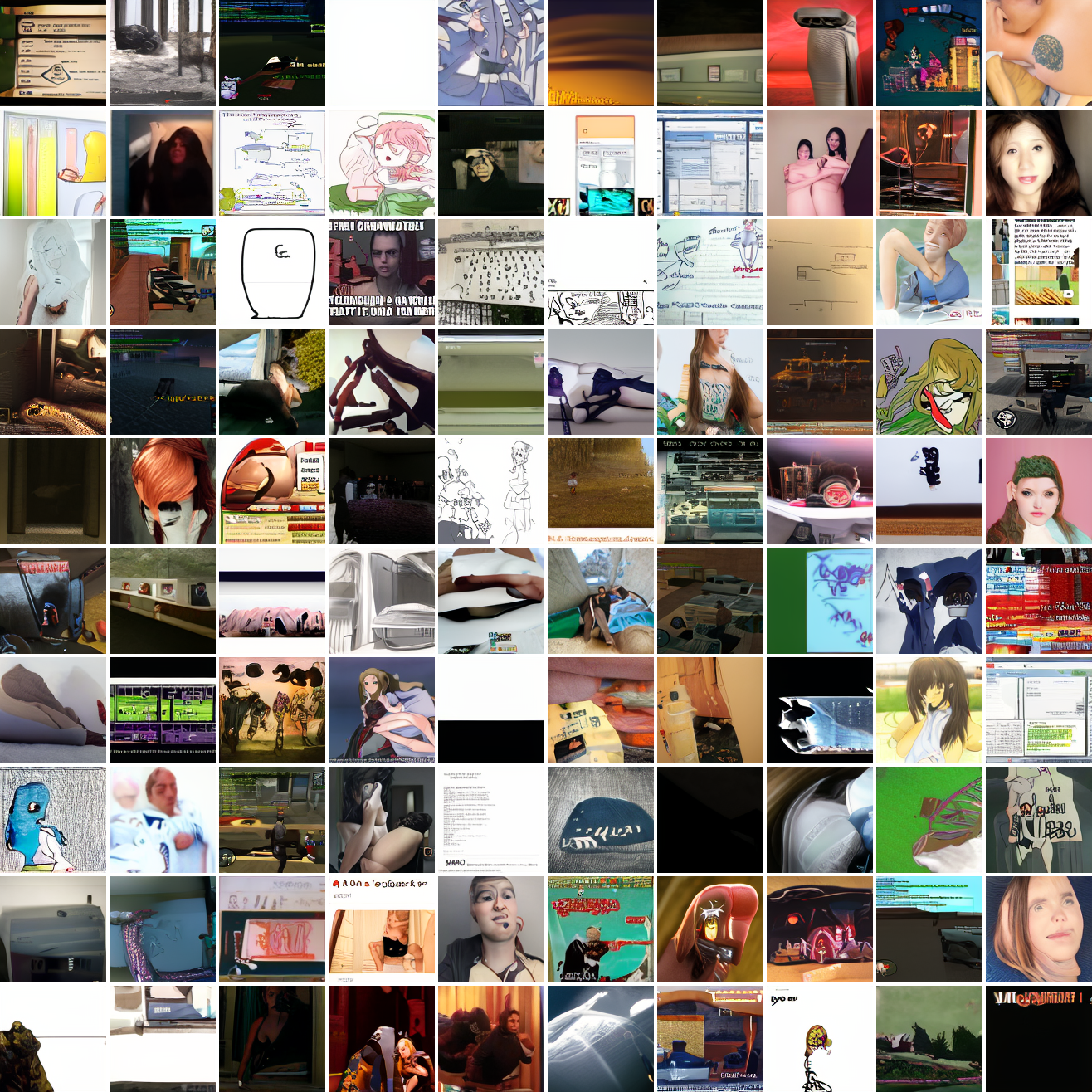
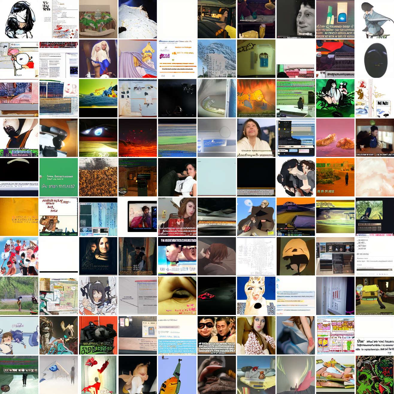
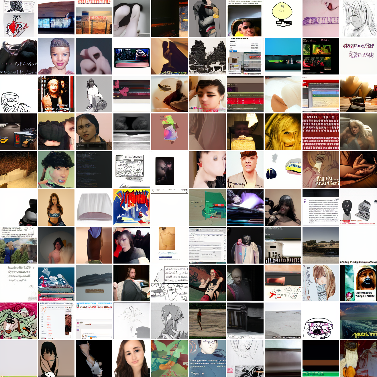
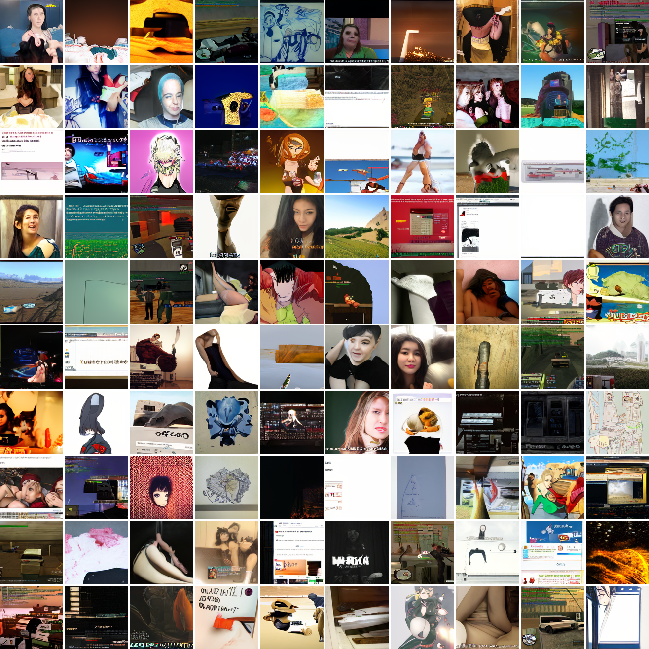
Here’s “a screenshot of Grand Theft Auto”:
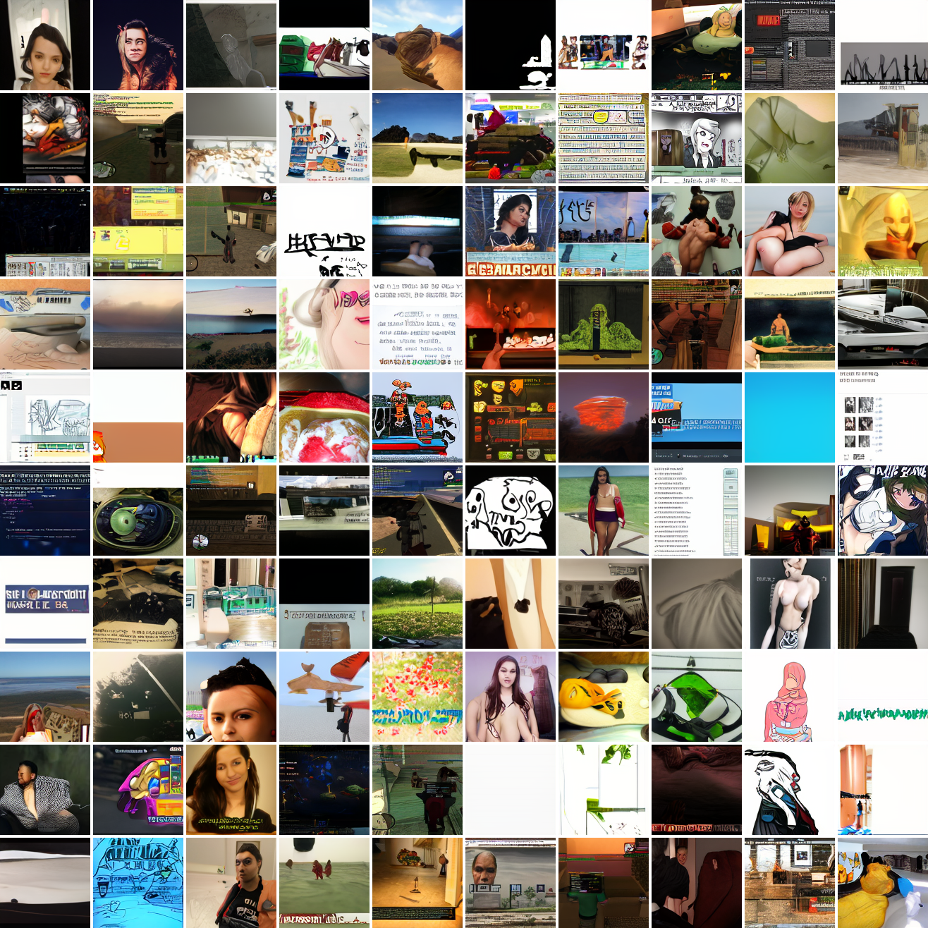
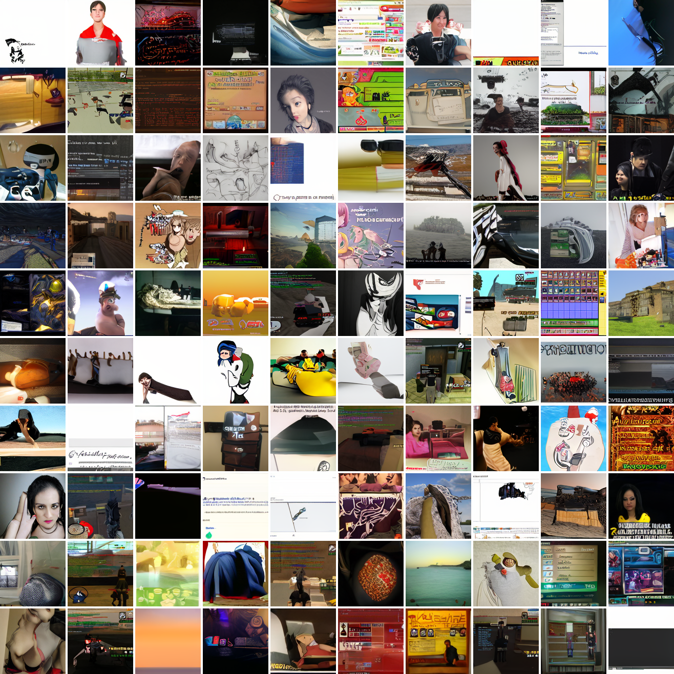
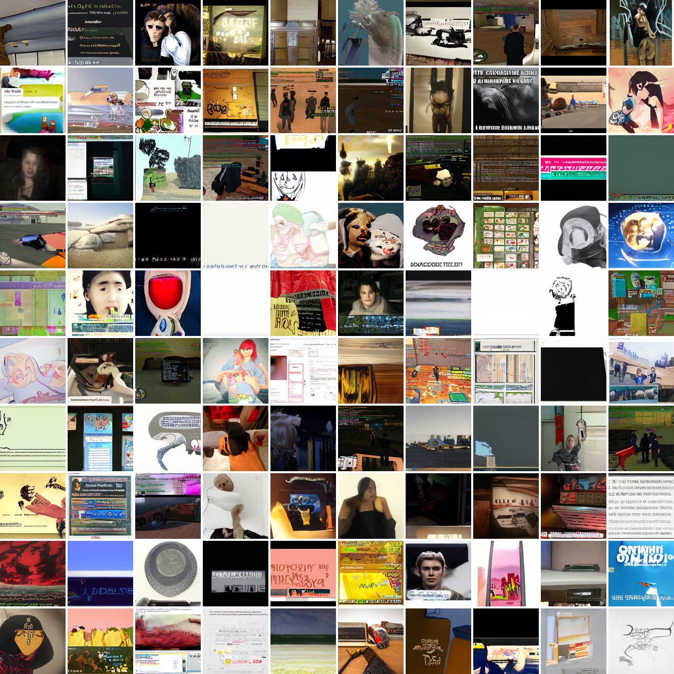
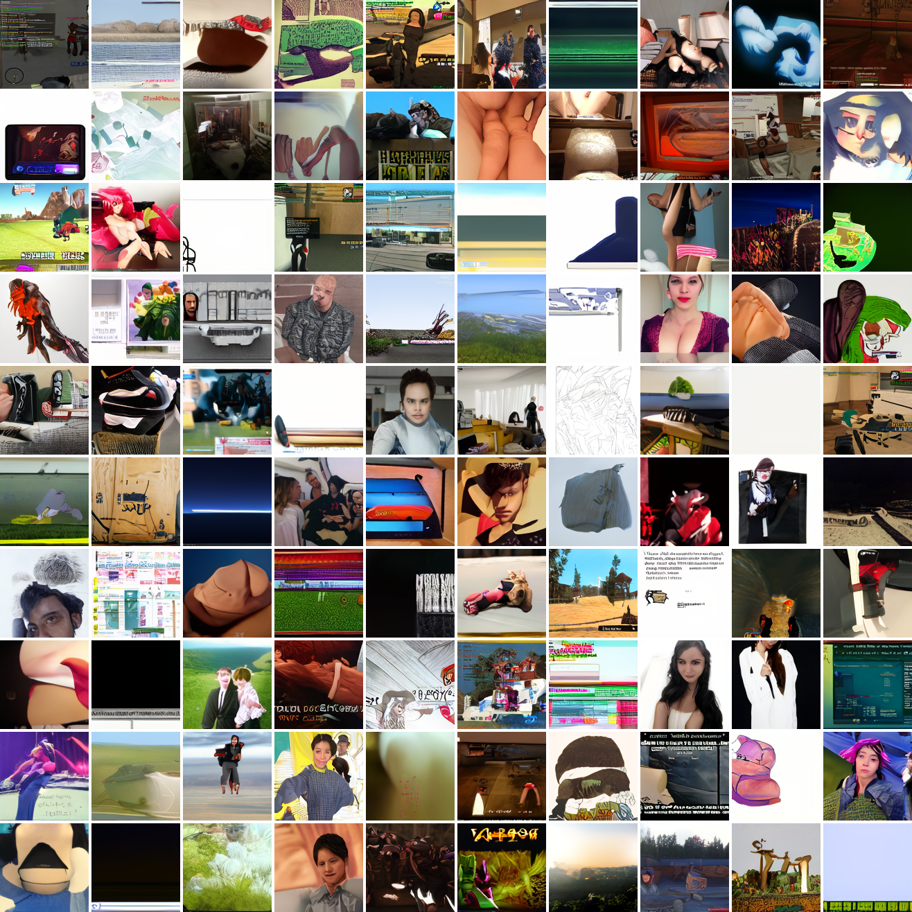
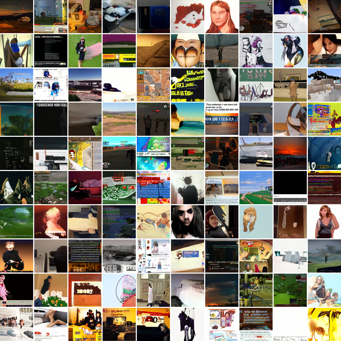
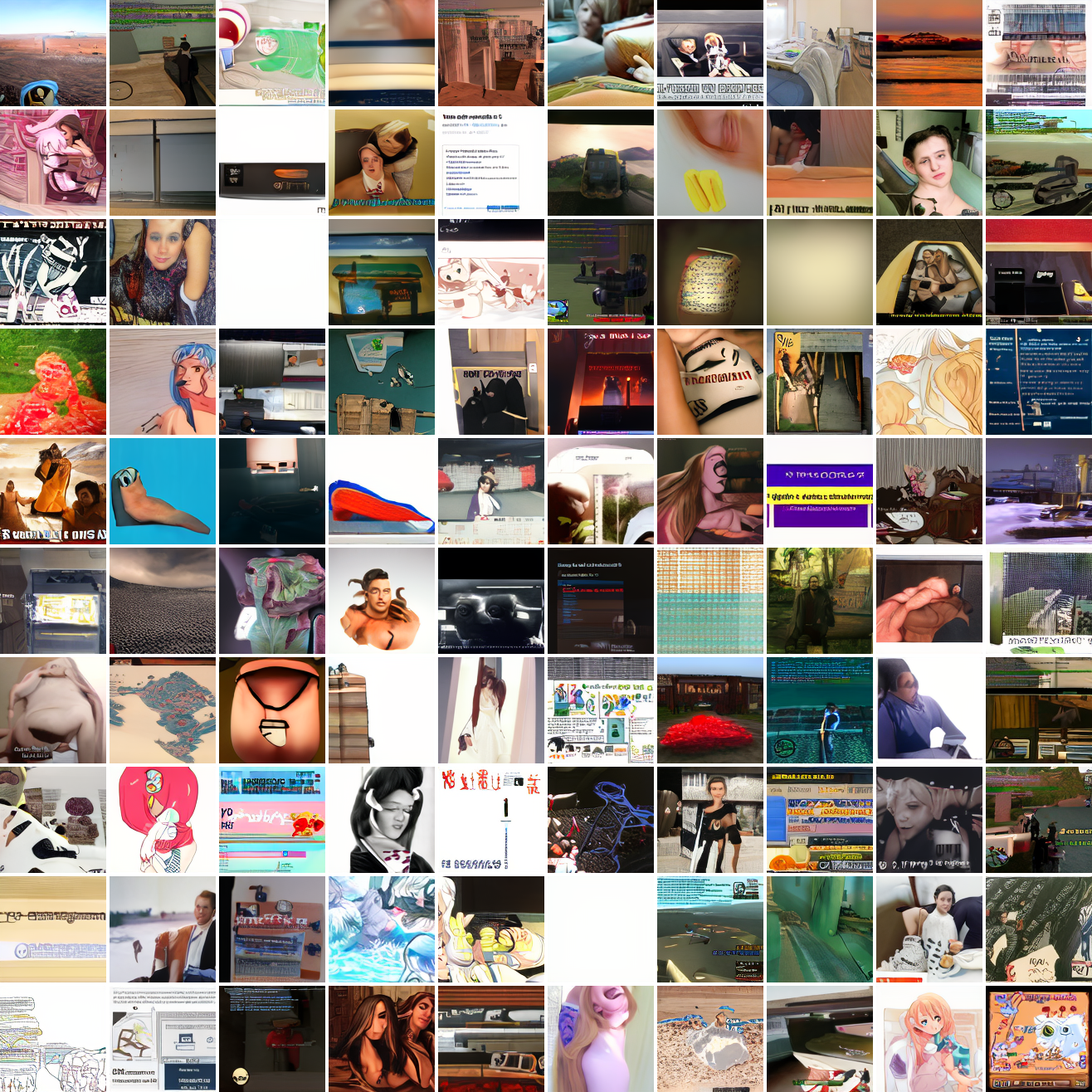
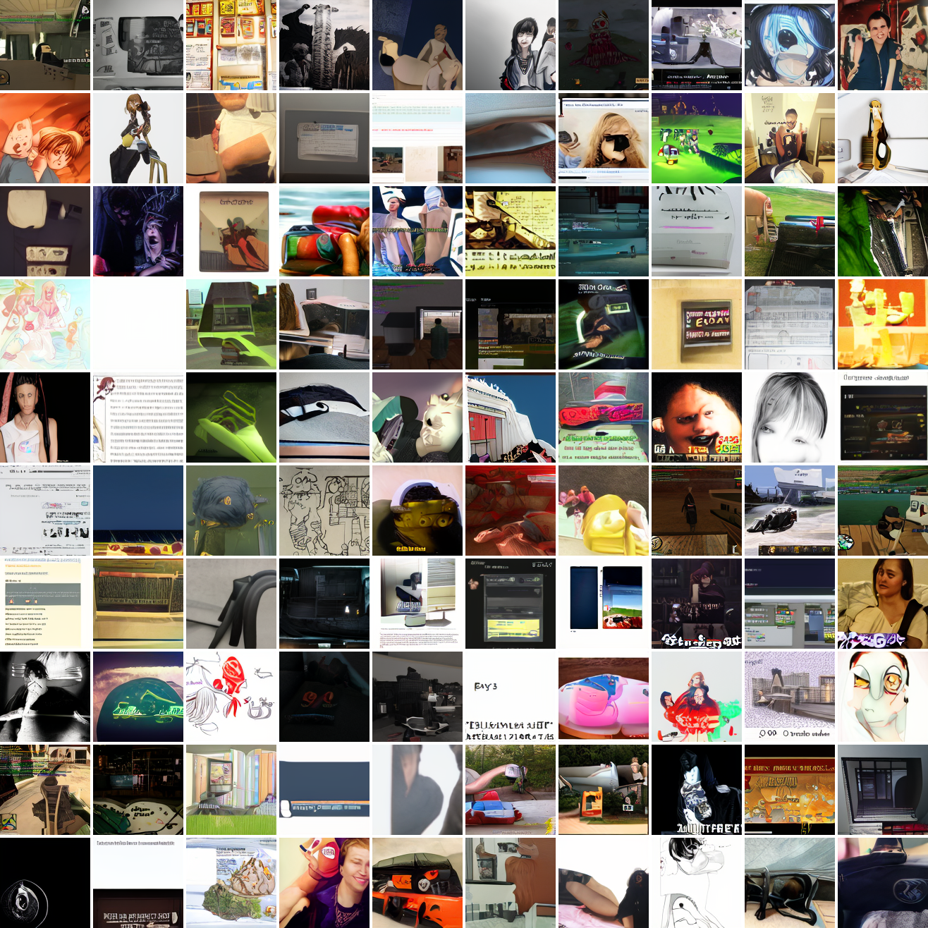
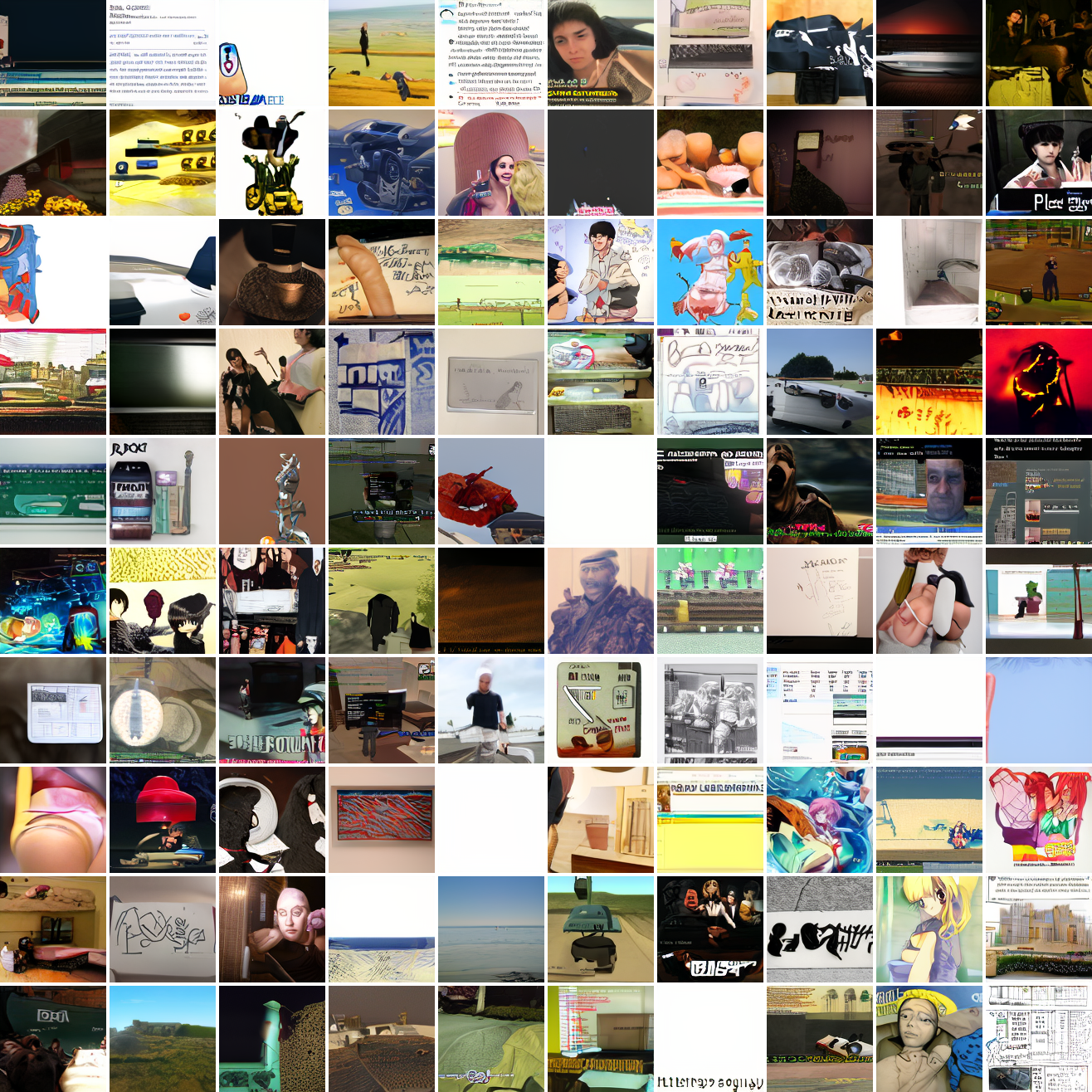
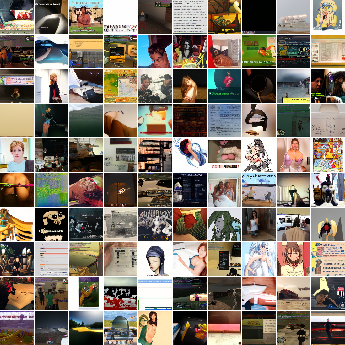
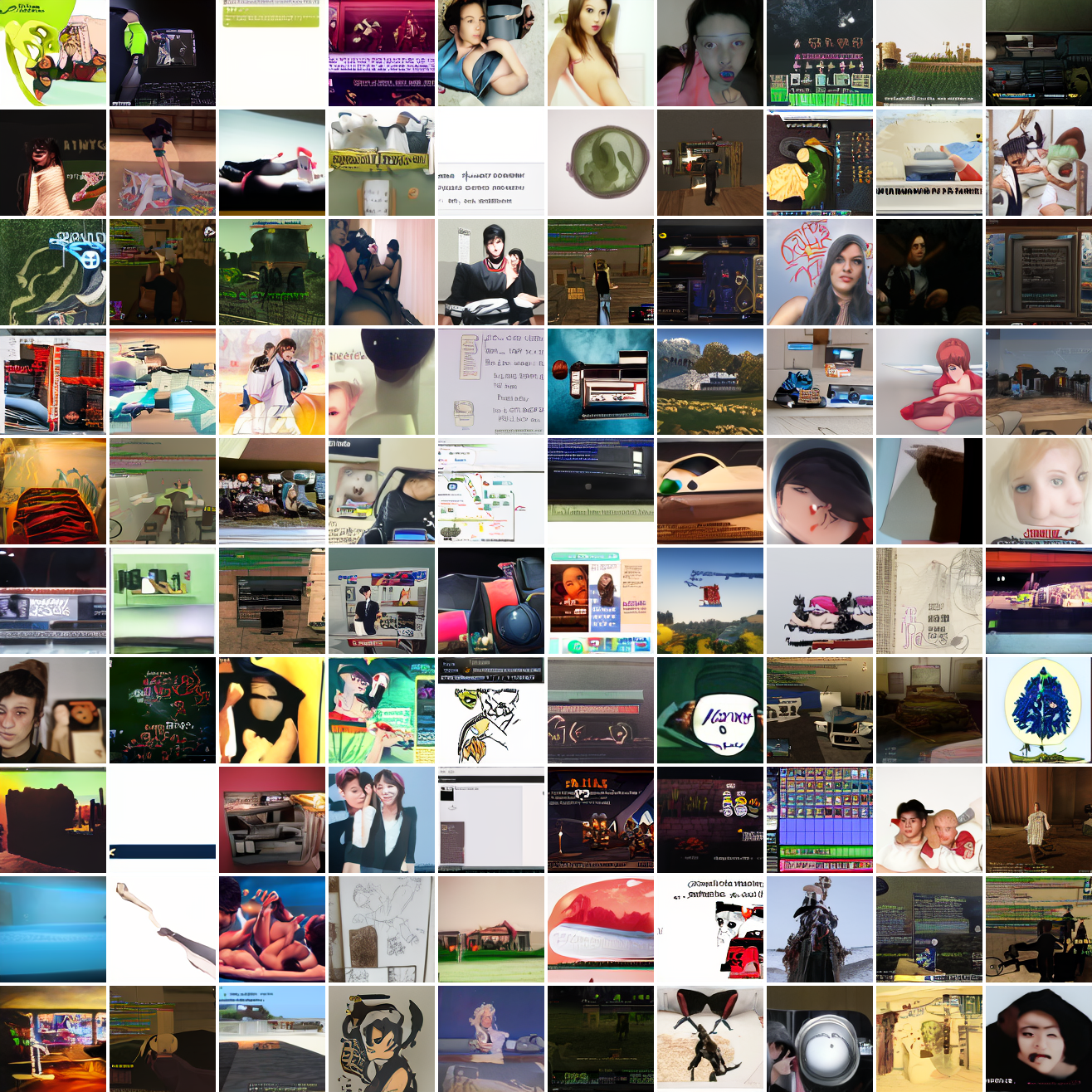
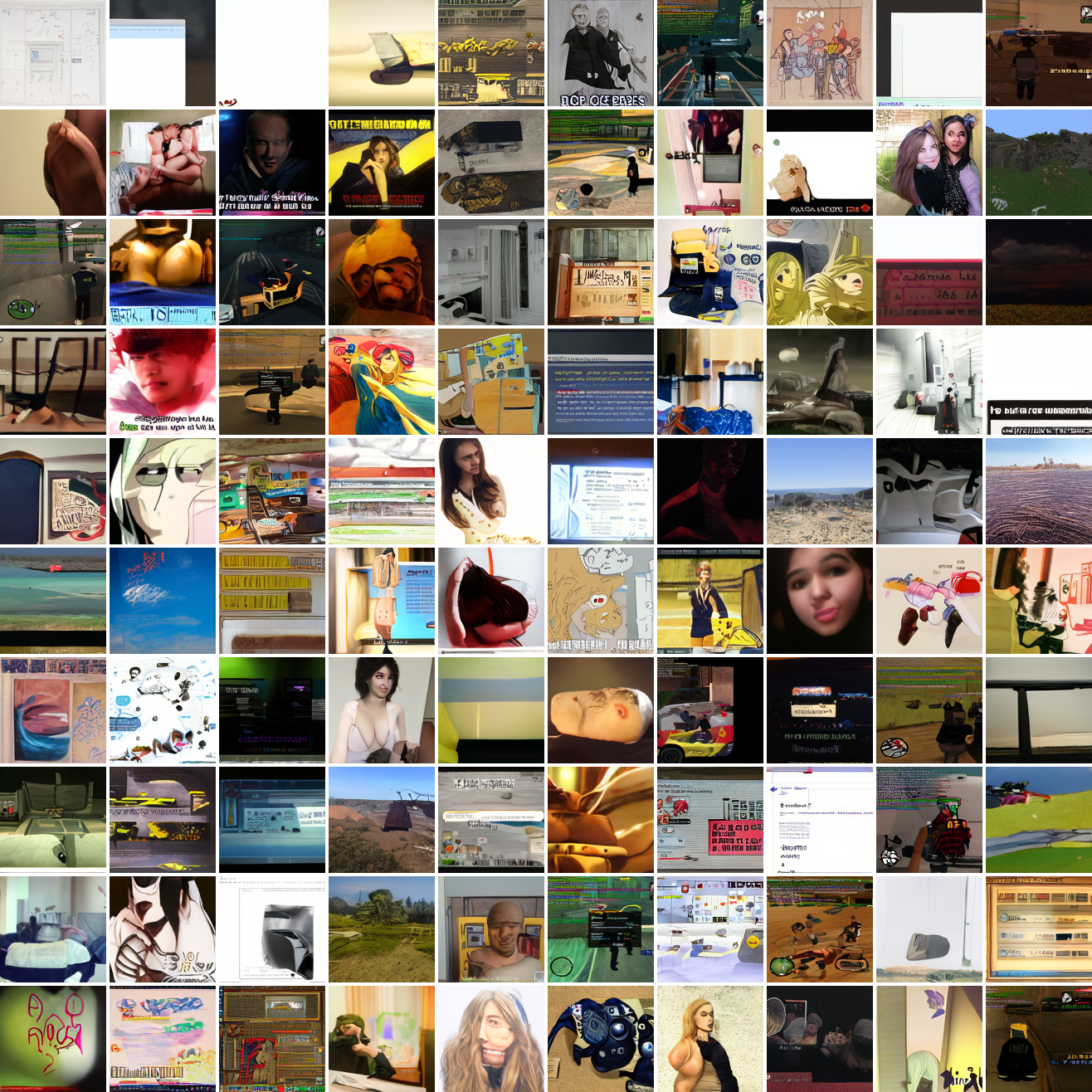
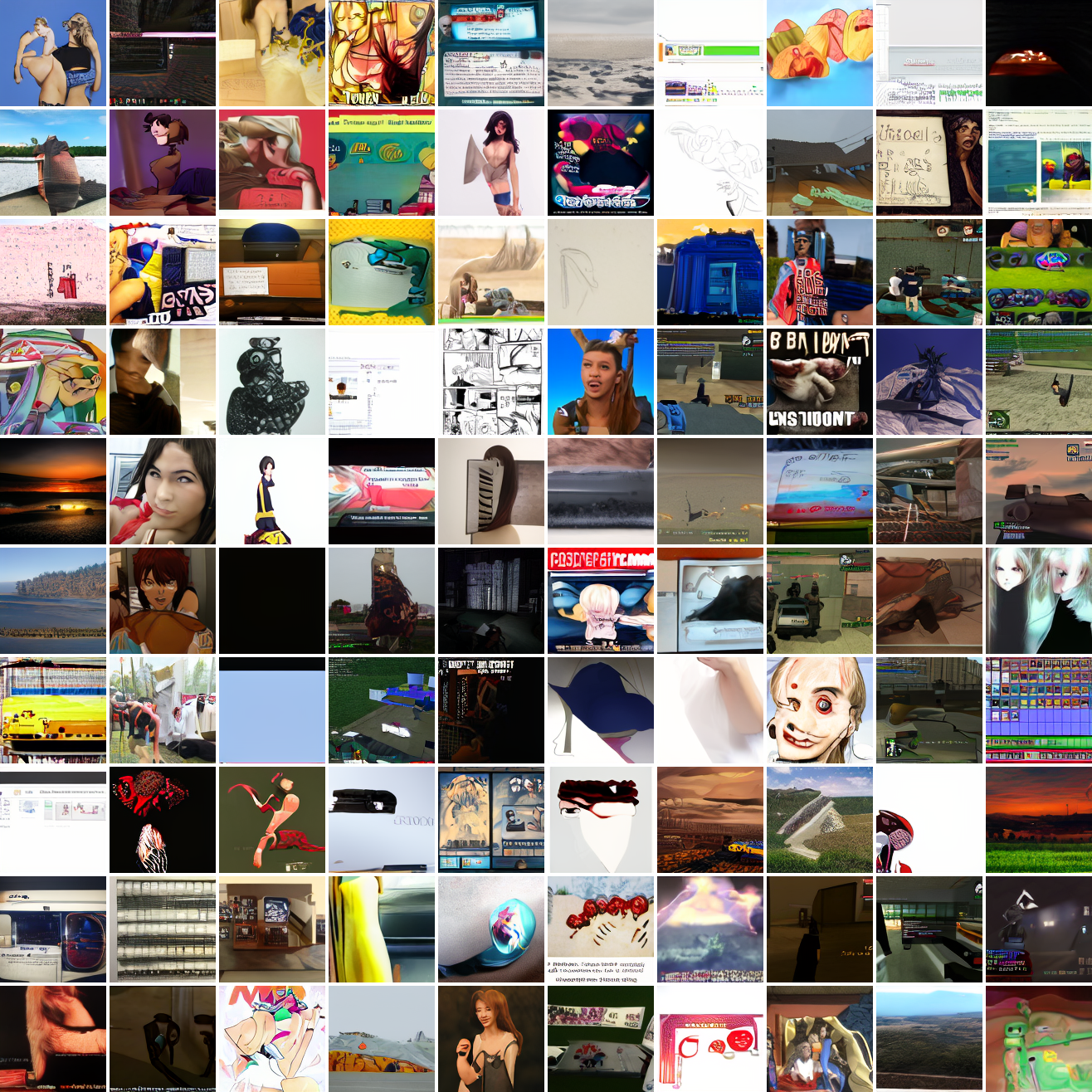
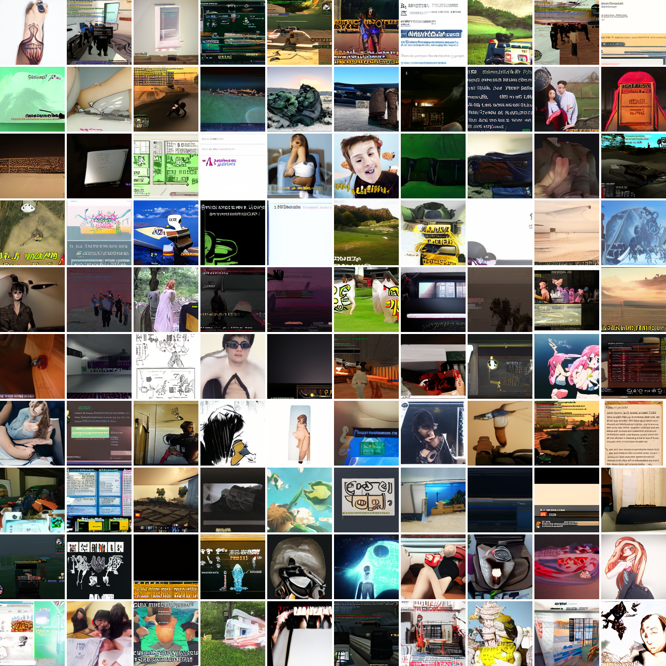
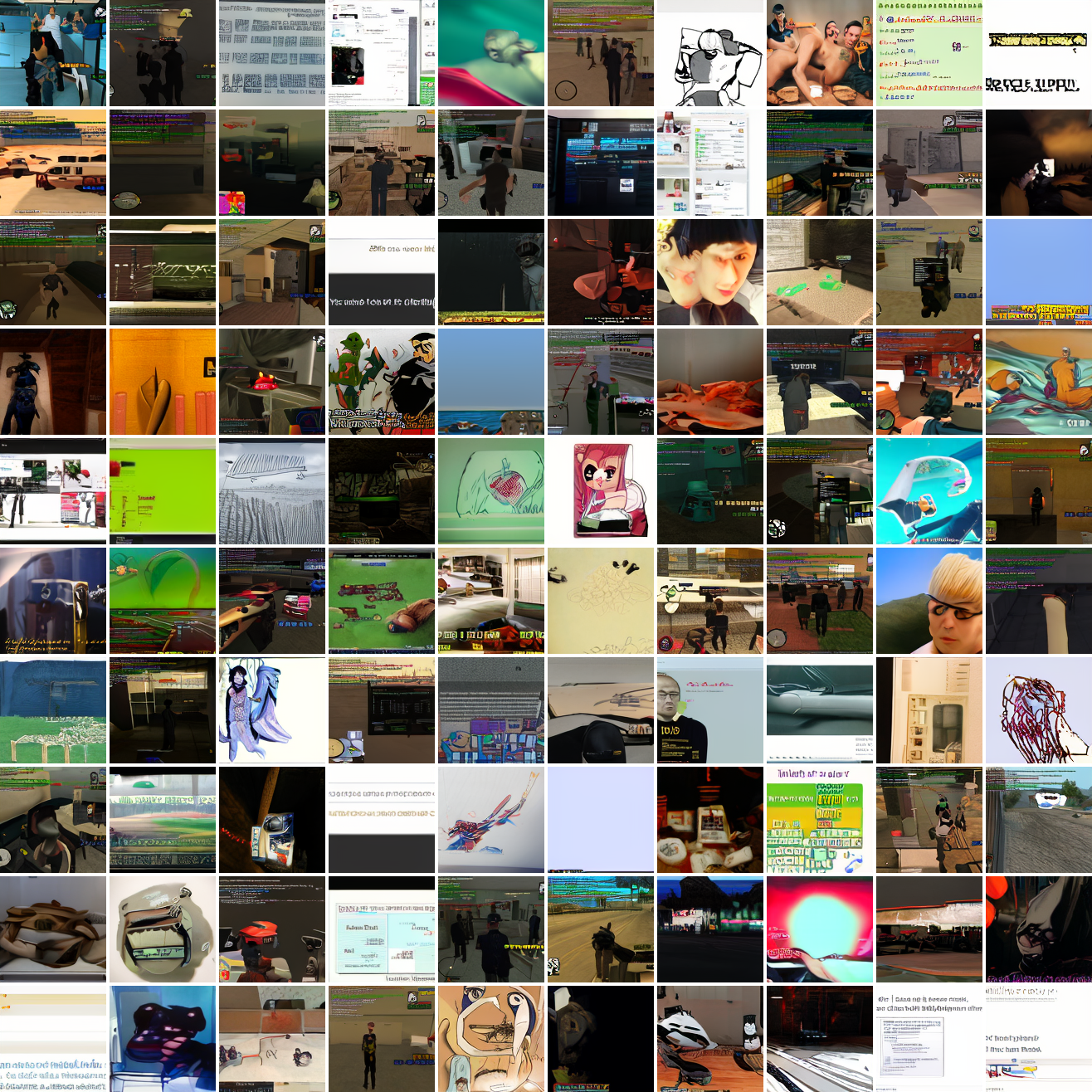
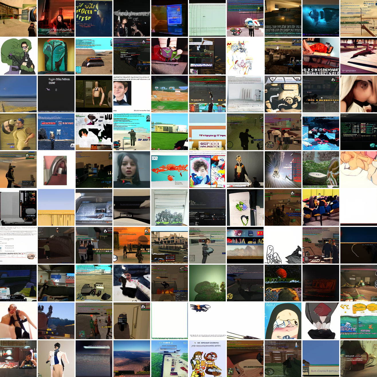
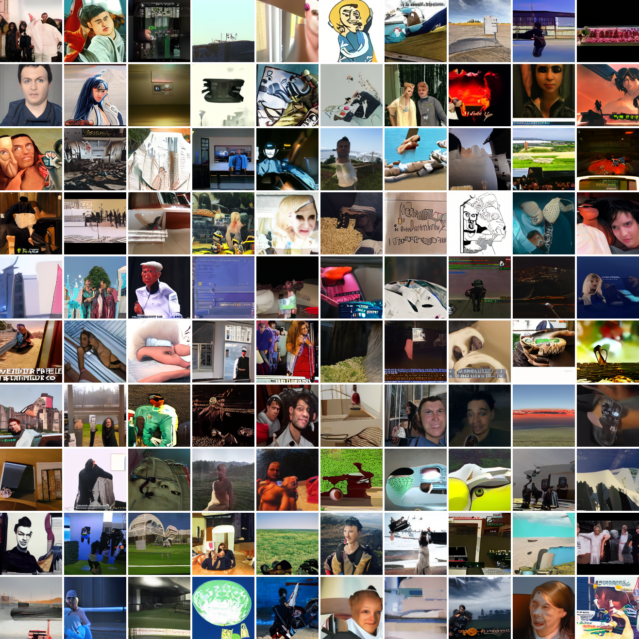
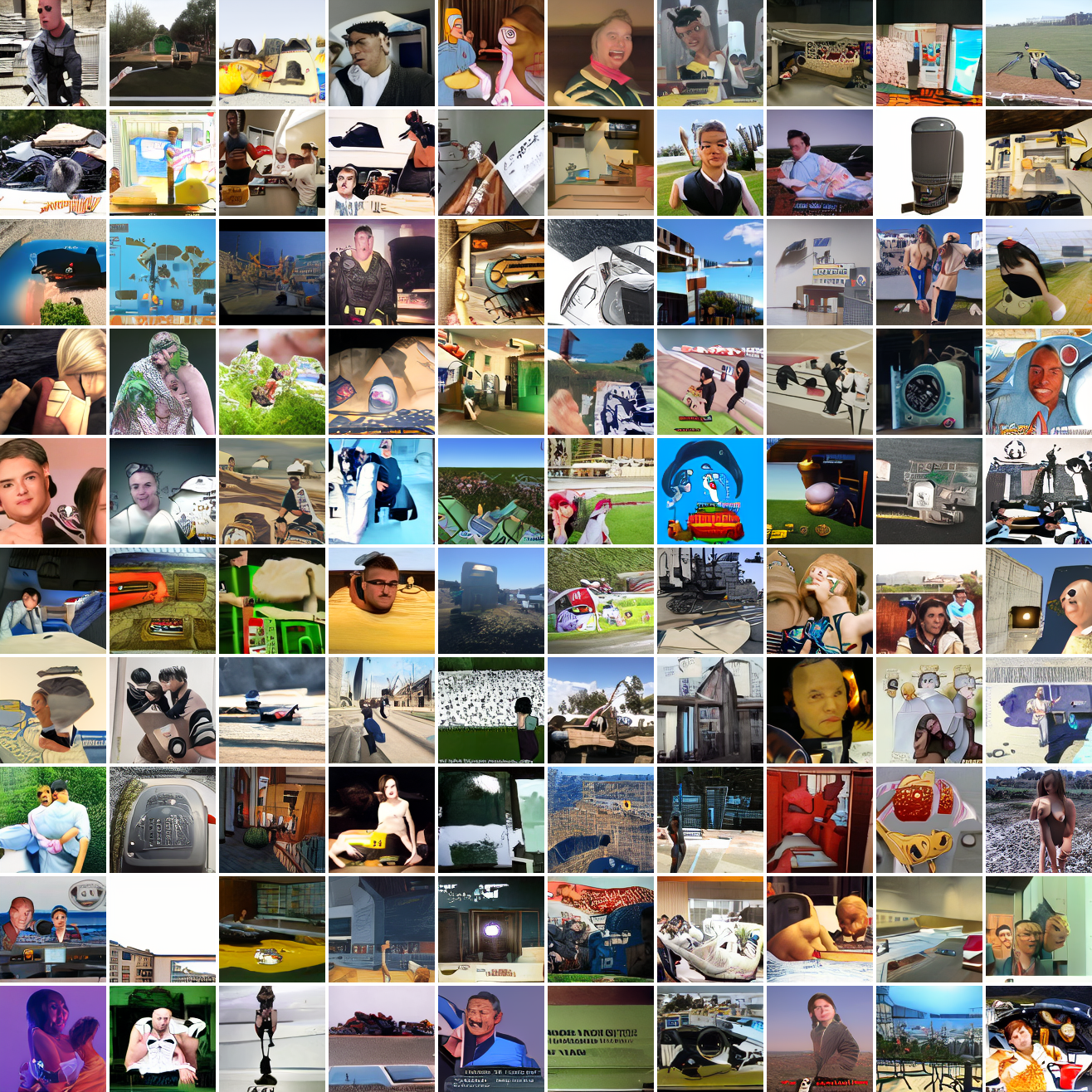
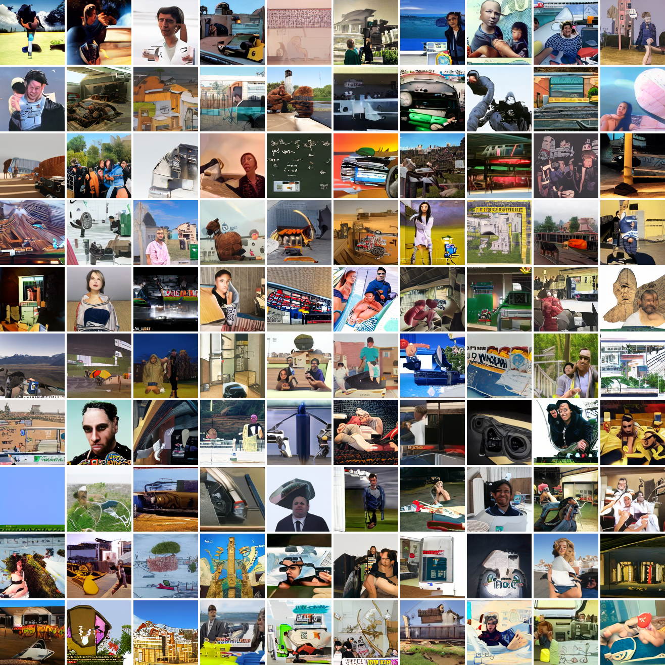
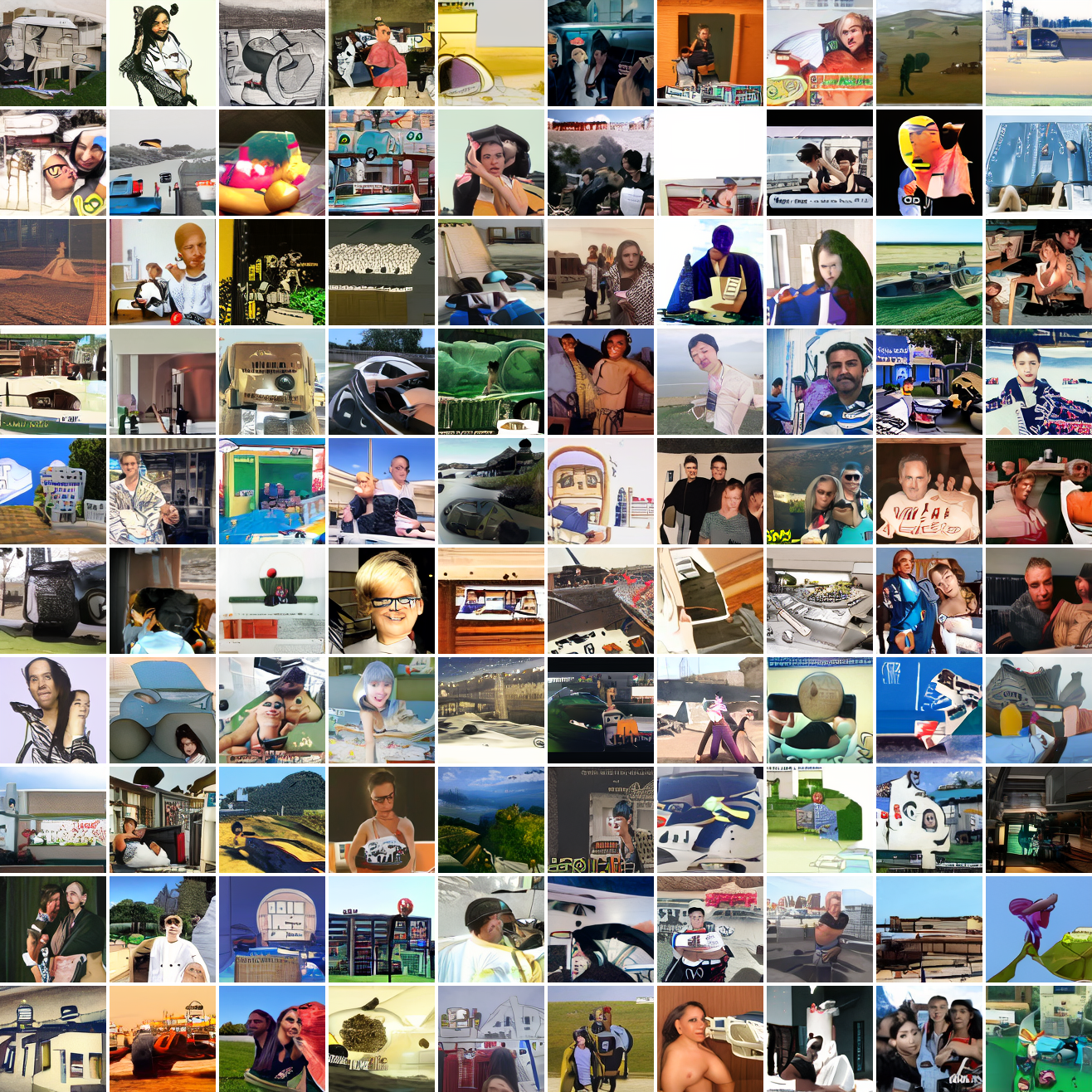
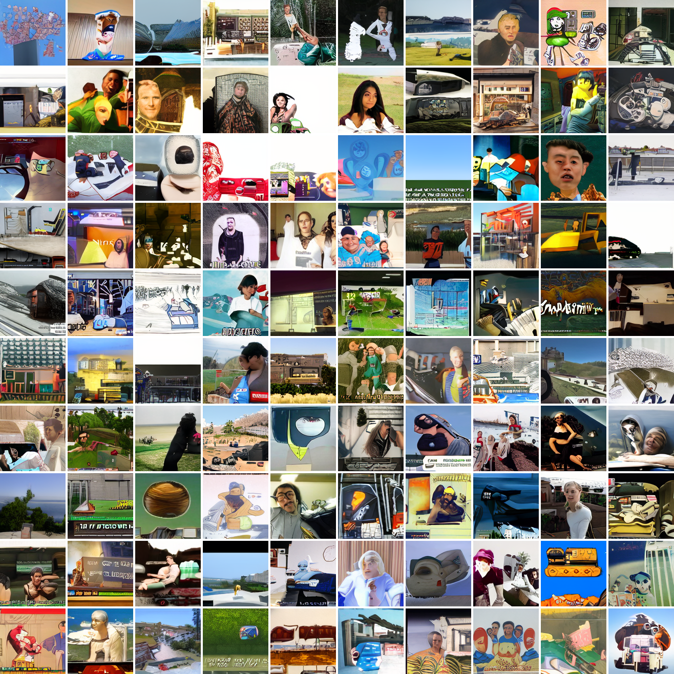
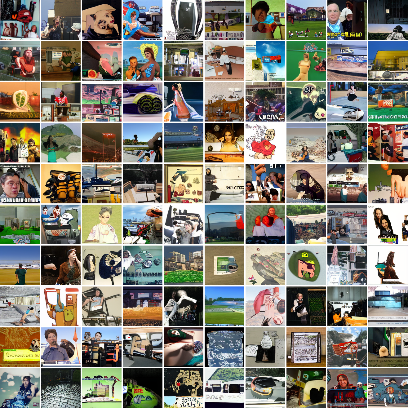
In both cases the fraction of images that resemble the prompt increases as the max cosine distance decreases. In the case of faces, there are high numbers of images that have faces in the range of 0.0 to 0.6 maximum cosine distance, but in the case of GTA screenshots, the range is more like 0.6 to 0.7. This makes some sense: the baseline model successfully generates faces when given an appropriate text prompt, but it can’t generate GTA screenshots from one. So we can suppose that there are images that have the same embedding as the text “A woman’s face”, but there aren’t images that have the same embedding as the text “A screenshot of Grand Theft Auto”. The cap conditioned model can only produce images that have embeddings inside a given cap if those images exist in the distribution.


The fraction of the images that resemble a GTA screenshot never exceeds 25%, and the fraction with faces never exceeds 64%. The model is undertrained, but I think this is actually decent proof of concept.
Next steps
Given all this, I’m reasonably confident this approach is sound. But as you saw in the samples, it doesn’t work very well yet. The simplest thing to do is scale up, training the model for longer, perhaps going up another notch in model size. It’d be much better to generate more cap-image pairs than to train for more epochs with the exact same pairs. And getting more data is of course always good. But I’ve seen very impressive results using comparable amounts of data to what I’m working with (the PixArt- guys brag about 33M), so that’s less of a priority.
Aside from model scale, I think it’d be worth messing with weighting the loss. The cap conditioned model mostly ignores the conditioning data at higher max cosine distances, and has similar loss to the baseline model, so I’m pretty sure that it’s mostly learning the unconditional distribution - predicting later image tokens from earlier ones and not from the conditioning token. It’s possible to counteract this by weighting the loss so that earlier tokens - where’s there’s less information from the image tokens and more from the conditioning token - are weighted more heavily. Worth experimenting with.
Another thing likely to improve quality is some kind of dataset balancing. It’s way too good at GTA screenshots relative to other stuff, and this is because they’re massively overrepresented in the dataset. On the other hand, it’s not that great at them so maybe better balancing would just get me a model that’s bad at everything.
This is a simplification. In reality, at each training step, there are n images and their n captions. The cosine similarities between each image’s embedding and each caption’s embedding are computed, then fed into a softmax, after a scaling factor is applied. The objective is to minimize cross entropy loss, and the scaling factor is learned. Anything I do with CLIP ignores the scaling factor and the softmax.↩︎
Both models are decoder only transformers generating 128x128 images, trained for one epoch on the 25 million image subset of my Imgur dataset that are sufficient resolution and are in RGB. The conditioning data is prepended to the sequence as a special token. The models generate sequences of 1024 tokens, which are fed into an autoencoder adapted from Latent Diffusion, which I ported to Jax/Flax, reusing their weights. The models use the middle size hyperparameters from the GPT-2 paper - 36 layers, d_model 1280, total parameters ~543M. The GPT-2 paper lists 762M in that configuration, and some of the difference is accounted for by the difference in vocabulary size (8192 vs 50,257). I’m not sure about the remainder. All samples are generated with top-p filtering with p=0.9. Models are trained with bf16 activations and f32 weights, and sampling is done with f32 activations.↩︎